Compute MxNE with time-frequency sparse prior

The TF-MxNE solver is a distributed inverse method (like dSPM or sLORETA) that promotes focal (sparse) sources (such as dipole fitting techniques) [1][2]. The benefit of this approach is that:

• it is spatio-temporal without assuming stationarity (sources properties can vary over time)

• activations are localized in space, time and frequency in one step.

• with a built-in filtering process based on a short time Fourier transform (STFT), data does not need to be low passed (just high pass to make the signals zero mean).

• the solver solves a convex optimization problem, hence cannot be trapped in local minima.

# Author: Alexandre Gramfort <alexandre.gramfort@inria.fr>
#         Daniel Strohmeier <daniel.strohmeier@tu-ilmenau.de>
#
# License: BSD-3-Clause
# Copyright the MNE-Python contributors.

import numpy as np

import mne
from mne.datasets import sample
from mne.inverse_sparse import make_stc_from_dipoles, tf_mixed_norm
from mne.minimum_norm import apply_inverse, make_inverse_operator
from mne.viz import (
    plot_dipole_amplitudes,
    plot_dipole_locations,
    plot_sparse_source_estimates,
)

print(__doc__)

data_path = sample.data_path()
subjects_dir = data_path / "subjects"
meg_path = data_path / "MEG" / "sample"
fwd_fname = meg_path / "sample_audvis-meg-eeg-oct-6-fwd.fif"
ave_fname = meg_path / "sample_audvis-no-filter-ave.fif"
cov_fname = meg_path / "sample_audvis-shrunk-cov.fif"

# Read noise covariance matrix
cov = mne.read_cov(cov_fname)

# Handling average file
condition = "Left visual"
evoked = mne.read_evokeds(ave_fname, condition=condition, baseline=(None, 0))
# We make the window slightly larger than what you'll eventually be interested
# in ([-0.05, 0.3]) to avoid edge effects.
evoked.crop(tmin=-0.1, tmax=0.4)

# Handling forward solution
forward = mne.read_forward_solution(fwd_fname)

    365 x 365 full covariance (kind = 1) found.
    Read a total of 4 projection items:
        PCA-v1 (1 x 102) active
        PCA-v2 (1 x 102) active
        PCA-v3 (1 x 102) active
        Average EEG reference (1 x 59) active
Reading /home/circleci/mne_data/MNE-sample-data/MEG/sample/sample_audvis-no-filter-ave.fif ...
    Read a total of 4 projection items:
        PCA-v1 (1 x 102) active
        PCA-v2 (1 x 102) active
        PCA-v3 (1 x 102) active
        Average EEG reference (1 x 60) active
    Found the data of interest:
        t =    -199.80 ...     499.49 ms (Left visual)
        0 CTF compensation matrices available
        nave = 64 - aspect type = 100
Projections have already been applied. Setting proj attribute to True.
Applying baseline correction (mode: mean)
Reading forward solution from /home/circleci/mne_data/MNE-sample-data/MEG/sample/sample_audvis-meg-eeg-oct-6-fwd.fif...
    Reading a source space...
    Computing patch statistics...
    Patch information added...
    Distance information added...
    [done]
    Reading a source space...
    Computing patch statistics...
    Patch information added...
    Distance information added...
    [done]
    2 source spaces read
    Desired named matrix (kind = 3523 (FIFF_MNE_FORWARD_SOLUTION_GRAD)) not available
    Read MEG forward solution (7498 sources, 306 channels, free orientations)
    Desired named matrix (kind = 3523 (FIFF_MNE_FORWARD_SOLUTION_GRAD)) not available
    Read EEG forward solution (7498 sources, 60 channels, free orientations)
    Forward solutions combined: MEG, EEG
    Source spaces transformed to the forward solution coordinate frame

Run solver

# alpha parameter is between 0 and 100 (100 gives 0 active source)
alpha = 40.0  # general regularization parameter
# l1_ratio parameter between 0 and 1 promotes temporal smoothness
# (0 means no temporal regularization)
l1_ratio = 0.03  # temporal regularization parameter

loose, depth = 0.2, 0.9  # loose orientation & depth weighting

# Compute dSPM solution to be used as weights in MxNE
inverse_operator = make_inverse_operator(
    evoked.info, forward, cov, loose=loose, depth=depth
)
stc_dspm = apply_inverse(evoked, inverse_operator, lambda2=1.0 / 9.0, method="dSPM")

# Compute TF-MxNE inverse solution with dipole output
dipoles, residual = tf_mixed_norm(
    evoked,
    forward,
    cov,
    alpha=alpha,
    l1_ratio=l1_ratio,
    loose=loose,
    depth=depth,
    maxit=200,
    tol=1e-6,
    weights=stc_dspm,
    weights_min=8.0,
    debias=True,
    wsize=16,
    tstep=4,
    window=0.05,
    return_as_dipoles=True,
    return_residual=True,
)

# Crop to remove edges
for dip in dipoles:
    dip.crop(tmin=-0.05, tmax=0.3)
evoked.crop(tmin=-0.05, tmax=0.3)
residual.crop(tmin=-0.05, tmax=0.3)

Converting forward solution to surface orientation
    Average patch normals will be employed in the rotation to the local surface coordinates....
    Converting to surface-based source orientations...
    [done]
info["bads"] and noise_cov["bads"] do not match, excluding bad channels from both
Computing inverse operator with 364 channels.
    364 out of 366 channels remain after picking
Selected 364 channels
Creating the depth weighting matrix...
    203 planar channels
    limit = 7262/7498 = 10.020865
    scale = 2.58122e-08 exp = 0.9
Applying loose dipole orientations to surface source spaces: 0.2
Whitening the forward solution.
    Created an SSP operator (subspace dimension = 4)
Computing rank from covariance with rank=None
    Using tolerance 3.5e-13 (2.2e-16 eps * 305 dim * 5.2  max singular value)
    Estimated rank (mag + grad): 302
    MEG: rank 302 computed from 305 data channels with 3 projectors
    Using tolerance 1.1e-13 (2.2e-16 eps * 59 dim * 8.7  max singular value)
    Estimated rank (eeg): 58
    EEG: rank 58 computed from 59 data channels with 1 projector
    Setting small MEG eigenvalues to zero (without PCA)
    Setting small EEG eigenvalues to zero (without PCA)
Creating the source covariance matrix
Adjusting source covariance matrix.
Computing SVD of whitened and weighted lead field matrix.
    largest singular value = 5.96729
    scaling factor to adjust the trace = 9.38524e+18 (nchan = 364 nzero = 4)
Preparing the inverse operator for use...
    Scaled noise and source covariance from nave = 1 to nave = 64
    Created the regularized inverter
    Created an SSP operator (subspace dimension = 4)
    Created the whitener using a noise covariance matrix with rank 360 (4 small eigenvalues omitted)
    Computing noise-normalization factors (dSPM)...
[done]
Applying inverse operator to "Left visual"...
    Picked 364 channels from the data
    Computing inverse...
    Eigenleads need to be weighted ...
    Computing residual...
    Explained  60.0% variance
    Combining the current components...
    dSPM...
[done]
Converting forward solution to surface orientation
    Average patch normals will be employed in the rotation to the local surface coordinates....
    Converting to surface-based source orientations...
    [done]
info["bads"] and noise_cov["bads"] do not match, excluding bad channels from both
Computing inverse operator with 364 channels.
    364 out of 366 channels remain after picking
Selected 364 channels
Creating the depth weighting matrix...
Applying loose dipole orientations to surface source spaces: 0.2
Whitening the forward solution.
    Created an SSP operator (subspace dimension = 4)
Computing rank from covariance with rank=None
    Using tolerance 3.5e-13 (2.2e-16 eps * 305 dim * 5.2  max singular value)
    Estimated rank (mag + grad): 302
    MEG: rank 302 computed from 305 data channels with 3 projectors
    Using tolerance 1.1e-13 (2.2e-16 eps * 59 dim * 8.7  max singular value)
    Estimated rank (eeg): 58
    EEG: rank 58 computed from 59 data channels with 1 projector
    Setting small MEG eigenvalues to zero (without PCA)
    Setting small EEG eigenvalues to zero (without PCA)
Creating the source covariance matrix
Adjusting source covariance matrix.
Reducing source space to 985 sources
Whitening data matrix.
Using block coordinate descent with active set approach

    Iteration 10 :: n_active 3
    dgap 3.49e+00 :: p_obj 4411.8457255277945 :: d_obj 4408.353440672169

    Iteration 20 :: n_active 3
    dgap 5.67e-01 :: p_obj 4410.859492179696 :: d_obj 4410.292945587401

dgap 1.51e-01 :: p_obj 4410.670058 :: d_obj 4410.519426 :: n_active 2

    Iteration 10 :: n_active 2
    dgap 1.61e-03 :: p_obj 4410.669663490567 :: d_obj 4410.668049322315

dgap 1.61e-03 :: p_obj 4410.669663 :: d_obj 4410.668049 :: n_active 2

Convergence reached!

Debiasing converged after 190 iterations max(|D - D0| = 5.547914e-07 < 1.000000e-06)
[done]

	General
	Filename(s)	sample_audvis-no-filter-ave.fif
	MNE object type	Evoked
	Measurement date	2002-12-03 at 19:01:10 UTC
	Participant	Unknown
	Experimenter	Unknown
	Acquisition
	Aggregation	average of 64 epochs
	Condition	Left visual
	Time range	-0.050 – 0.300 s
	Baseline	-0.200 – 0.000 s
	Sampling frequency	600.61 Hz
	Time points	211
	Channels
	Magnetometers	102
	Gradiometers	203
	EEG	59
	Head & sensor digitization	146 points
	Filters
	Highpass	0.10 Hz
	Lowpass	172.18 Hz
	Projections	PCA-v1 (on) PCA-v2 (on) PCA-v3 (on) Average EEG reference (on)

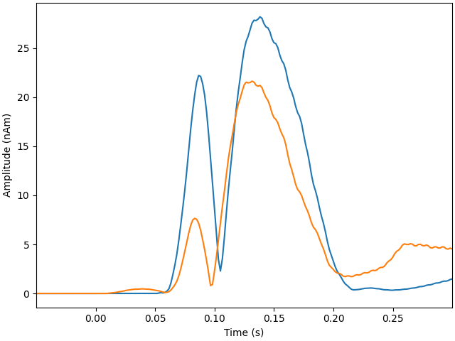
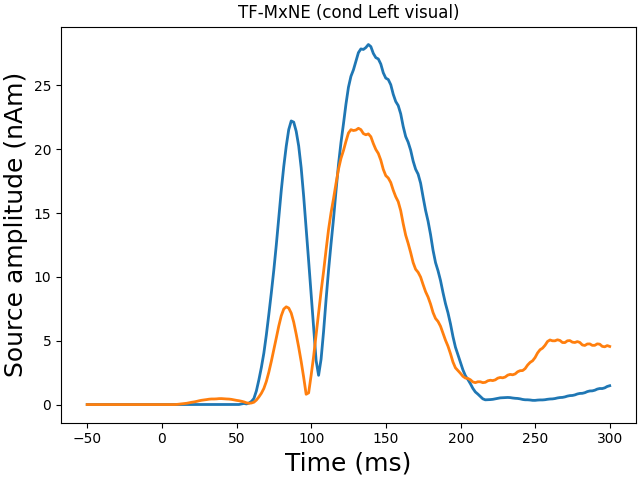
Plot dipole activations

plot_dipole_amplitudes(dipoles)

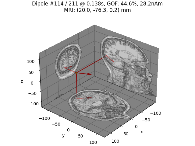
Plot location of the strongest dipole with MRI slices

idx = np.argmax([np.max(np.abs(dip.amplitude)) for dip in dipoles])
plot_dipole_locations(
    dipoles[idx],
    forward["mri_head_t"],
    "sample",
    subjects_dir=subjects_dir,
    mode="orthoview",
    idx="amplitude",
)

# # Plot dipole locations of all dipoles with MRI slices:
# for dip in dipoles:
#     plot_dipole_locations(dip, forward['mri_head_t'], 'sample',
#                           subjects_dir=subjects_dir, mode='orthoview',
#                           idx='amplitude')

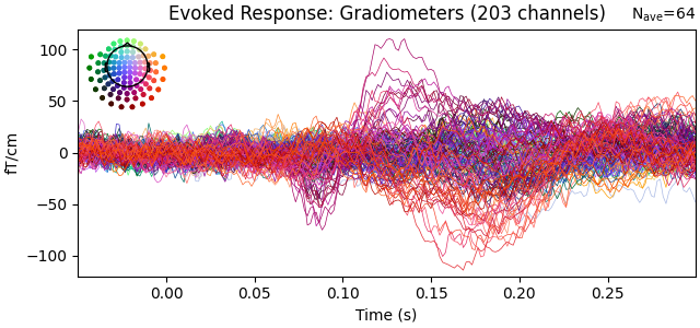
Show the evoked response and the residual for gradiometers

ylim = dict(grad=[-120, 120])
evoked.pick(picks="grad", exclude="bads")
evoked.plot(
    titles=dict(grad="Evoked Response: Gradiometers"),
    ylim=ylim,
    proj=True,
    time_unit="s",
)

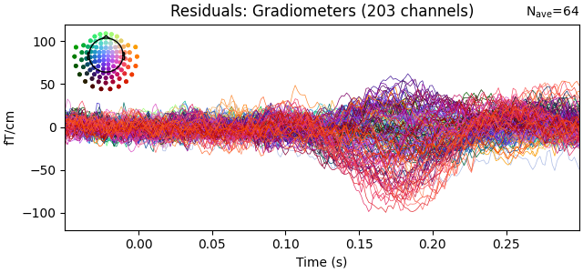
residual.pick(picks="grad", exclude="bads")
residual.plot(
    titles=dict(grad="Residuals: Gradiometers"), ylim=ylim, proj=True, time_unit="s"
)

• 
• 

Generate stc from dipoles

stc = make_stc_from_dipoles(dipoles, forward["src"])

Converting dipoles into a SourceEstimate.
[done]

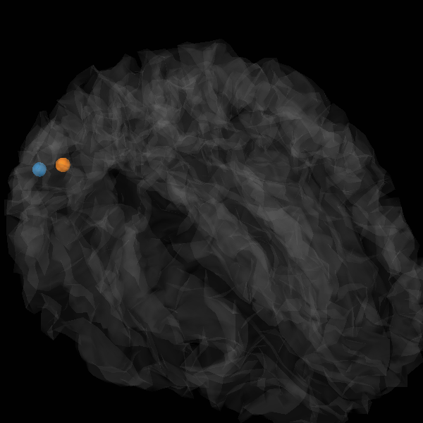
View in 2D and 3D (“glass” brain like 3D plot)

plot_sparse_source_estimates(
    forward["src"],
    stc,
    bgcolor=(1, 1, 1),
    opacity=0.1,
    fig_name=f"TF-MxNE (cond {condition})",
    modes=["sphere"],
    scale_factors=[1.0],
)

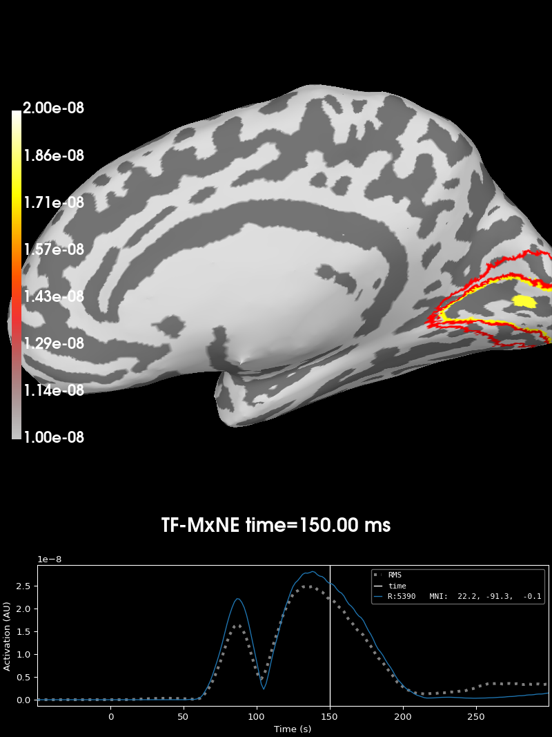
time_label = "TF-MxNE time=%0.2f ms"
clim = dict(kind="value", lims=[10e-9, 15e-9, 20e-9])
brain = stc.plot(
    "sample",
    "inflated",
    "rh",
    views="medial",
    clim=clim,
    time_label=time_label,
    smoothing_steps=5,
    subjects_dir=subjects_dir,
    initial_time=150,
    time_unit="ms",
)
brain.add_label("V1", color="yellow", scalar_thresh=0.5, borders=True)
brain.add_label("V2", color="red", scalar_thresh=0.5, borders=True)

Total number of active sources: [160797 167557]

References

[1]

Alexandre Gramfort, Daniel T. Strohmeier, Jens Haueisen, Matti S. Hämäläinen, and Matthieu Kowalski. Time-frequency mixed-norm estimates: sparse M/EEG imaging with non-stationary source activations. NeuroImage, 70:410–422, 2013. doi:10.1016/j.neuroimage.2012.12.051.

[2]

Alexandre Gramfort, Daniel Strohmeier, Jens Haueisen, Matti S. Hämäläinen, and Matthieu Kowalski. Functional brain imaging with M/EEG using structured sparsity in time-frequency dictionaries. In Gábor Székely and Horst K. Hahn, editors, Information Processing in Medical Imaging, volume 6801, pages 600–611. Springer, Berlin; Heidelberg, 2011. doi:10.1007/978-3-642-22092-0_49.