Note
Go to the end to download the full example code.
Visualizing epoched data#
This tutorial shows how to plot epoched data as time series, how to plot the
spectral density of epoched data, how to plot epochs as an imagemap, and how to
plot the sensor locations and projectors stored in Epochs objects.
We’ll start by importing the modules we need, loading the continuous (raw) sample data, and cropping it to save memory:
# Authors: The MNE-Python contributors.
# License: BSD-3-Clause
# Copyright the MNE-Python contributors.
import mne

sample_data_folder = mne.datasets.sample.data_path()
sample_data_raw_file = sample_data_folder / "MEG" / "sample" / "sample_audvis_raw.fif"
raw = mne.io.read_raw_fif(sample_data_raw_file, verbose=False).crop(tmax=120)
To create the Epochs data structure, we’ll extract the event IDs stored in the
stim channel, map those integer event IDs to more descriptive condition labels
using an event dictionary, and pass those to the Epochs constructor, along with
the Raw data and the desired temporal limits of our epochs, tmin and
tmax (for a detailed explanation of these steps, see The Epochs data structure: discontinuous data).
events = mne.find_events(raw, stim_channel="STI 014")
event_dict = {
    "auditory/left": 1,
    "auditory/right": 2,
    "visual/left": 3,
    "visual/right": 4,
    "face": 5,
    "button": 32,
}
epochs = mne.Epochs(raw, events, tmin=-0.2, tmax=0.5, event_id=event_dict, preload=True)
del raw
Finding events on: STI 014
176 events found on stim channel STI 014
Event IDs: [ 1  2  3  4  5 32]
Not setting metadata
176 matching events found
Setting baseline interval to [-0.19979521315838786, 0.0] s
Applying baseline correction (mode: mean)
Created an SSP operator (subspace dimension = 3)
3 projection items activated
Loading data for 176 events and 421 original time points ...
1 bad epochs dropped
Plotting Epochs as time series#
To visualize epoched data as time series (one time series per channel), the
mne.Epochs.plot method is available. It creates an interactive window
where you can scroll through epochs and channels, enable/disable any
unapplied SSP projectors to see how they affect the
signal, and even manually mark bad channels (by clicking the channel name) or
bad epochs (by clicking the data) for later dropping. Channels marked “bad”
will be shown in light grey color and will be added to
epochs.info['bads']; epochs marked as bad will be indicated as 'USER'
in epochs.drop_log.
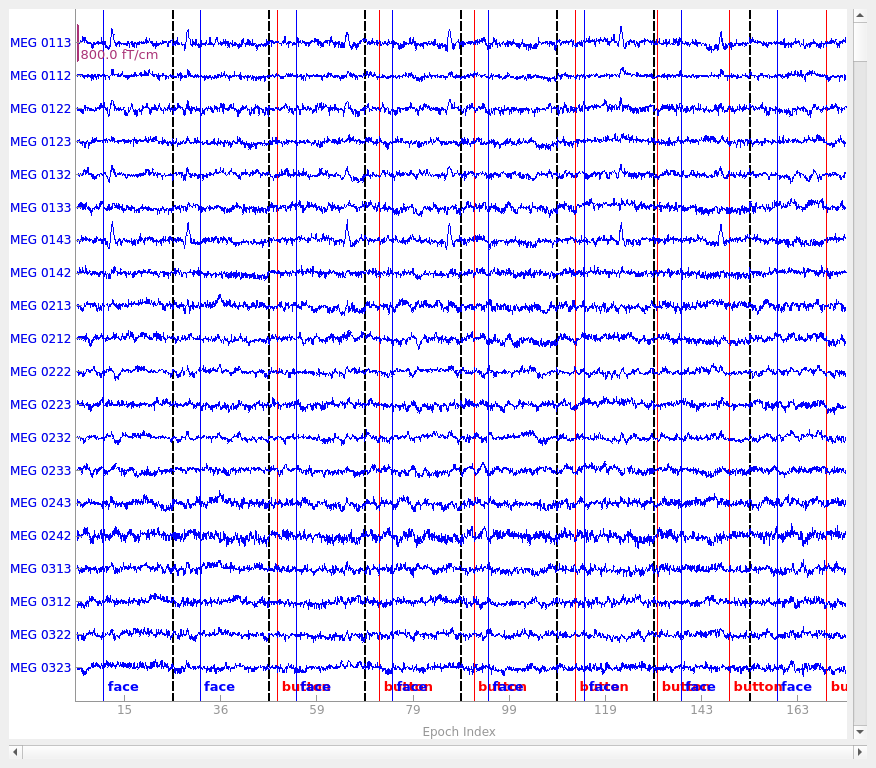
Here we’ll plot only the “catch” trials from the sample dataset, and pass in our events array so that the button press
responses also get marked (we’ll plot them in red, and plot the “face” events
defining time zero for each epoch in blue). We also need to pass in
our event_dict so that the plot method will know what
we mean by “button” — this is because subsetting the conditions by
calling epochs['face'] automatically purges the dropped entries from
epochs.event_id:
catch_trials_and_buttonpresses = mne.pick_events(events, include=[5, 32])
epochs["face"].plot(
    events=catch_trials_and_buttonpresses,
    event_id=event_dict,
    event_color=dict(button="red", face="blue"),
)
Using qt as 2D backend.
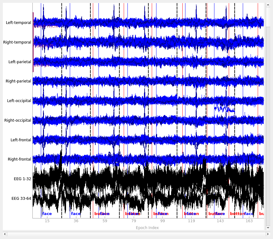
To see all sensors at once, we can use butterfly mode and group by selection:
epochs["face"].plot(
    events=catch_trials_and_buttonpresses,
    event_id=event_dict,
    event_color=dict(button="red", face="blue"),
    group_by="selection",
    butterfly=True,
)
Plotting projectors from an Epochs object#
In the plot above we can see heartbeat artifacts in the magnetometer channels, so before we continue let’s load ECG projectors from disk and apply them to the data:
ecg_proj_file = sample_data_folder / "MEG" / "sample" / "sample_audvis_ecg-proj.fif"
ecg_projs = mne.read_proj(ecg_proj_file)
epochs.add_proj(ecg_projs)
epochs.apply_proj()
    Read a total of 6 projection items:
        ECG-planar-999--0.200-0.400-PCA-01 (1 x 203)  idle
        ECG-planar-999--0.200-0.400-PCA-02 (1 x 203)  idle
        ECG-axial-999--0.200-0.400-PCA-01 (1 x 10²)  idle
        ECG-axial-999--0.200-0.400-PCA-02 (1 x 10²)  idle
        ECG-eeg-999--0.200-0.400-PCA-01 (1 x 59)  idle
        ECG-eeg-999--0.200-0.400-PCA-02 (1 x 59)  idle
6 projection items deactivated
Created an SSP operator (subspace dimension = 9)
9 projection items activated
SSP projectors applied...
Just as we saw in the Plotting projectors from Raw objects section, we can plot the
projectors present in an Epochs object using the same
plot_projs_topomap method. Since the original three empty-room
magnetometer projectors were inherited from the Raw file, and we added two
ECG projectors for each sensor type, we should see nine projector topomaps:
epochs.plot_projs_topomap(vlim="joint")
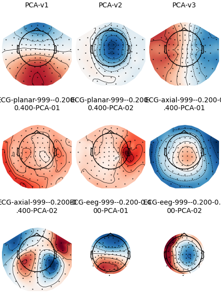
Note that these field maps illustrate aspects of the signal that have
already been removed (because projectors in Raw data are
applied by default when epoching, and because we called
apply_proj after adding additional ECG projectors from file).
You can check this by examining the 'active' field of the projectors:
print(all(proj["active"] for proj in epochs.info["projs"]))
True
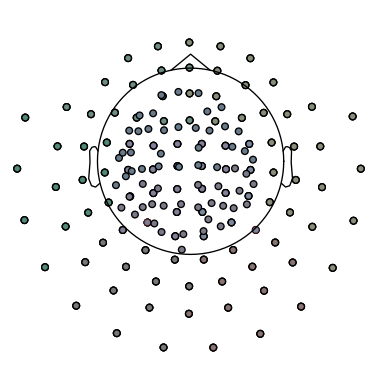
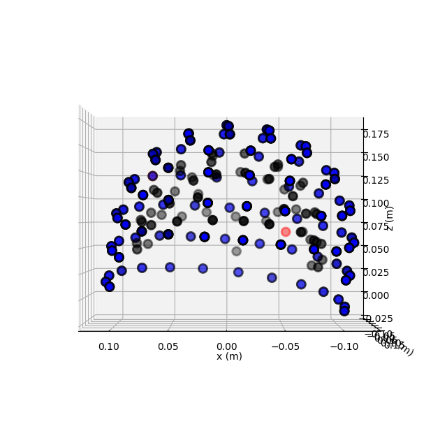
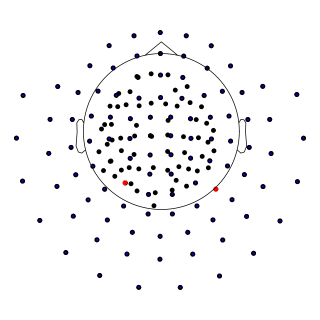
Plotting sensor locations#
Just like Raw objects, Epochs objects
keep track of sensor locations, which can be visualized with the
plot_sensors method:
epochs.plot_sensors(kind="3d", ch_type="all")
epochs.plot_sensors(kind="topomap", ch_type="all")
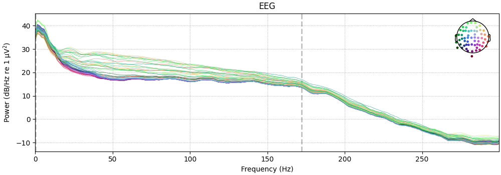
Plotting the power spectrum of Epochs#
Again, just like Raw objects, Epochs objects
can be converted to spectral density via
compute_psd(), which can then be plotted using the
EpochsSpectrum’s
plot() method.
epochs["auditory"].compute_psd().plot(picks="eeg", exclude="bads", amplitude=False)
    Using multitaper spectrum estimation with 7 DPSS windows
Plotting power spectral density (dB=True).
Averaging across epochs before plotting...
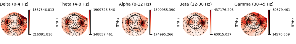
It is also possible to plot spectral power estimates across sensors as a
scalp topography, using the EpochsSpectrum’s
plot_topomap() method. The default
parameters will plot five frequency bands (δ, θ, α, β, γ), will compute power
based on magnetometer channels (if present), and will plot the power
estimates on a dB-like log-scale:
spectrum = epochs["visual/right"].compute_psd()
spectrum.plot_topomap()
    Using multitaper spectrum estimation with 7 DPSS windows
Averaging across epochs before plotting...
Note
Prior to the addition of the EpochsSpectrum
class, the above plots were possible via:
The plot_psd() and plot_psd_topomap
methods of Epochs objects are still provided to support
legacy analysis scripts, but new code should instead use the
EpochsSpectrum object API.
Just like plot_projs_topomap,
EpochsSpectrum.plot_topomap()
has a vlim='joint' option for fixing the colorbar limits jointly across
all subplots, to give a better sense of the relative magnitude in each
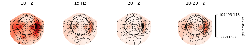
frequency band. You can change which channel type is used via the
ch_type parameter, and if you want to view different frequency bands than
the defaults, the bands parameter takes a dict, with keys
providing a subplot title and values providing either single frequency bins
to plot, or lower/upper frequency band edges:
bands = {"10 Hz": 10, "15 Hz": 15, "20 Hz": 20, "10-20 Hz": (10, 20)}
spectrum.plot_topomap(bands=bands, vlim="joint", ch_type="grad")
Averaging across epochs before plotting...
If you prefer untransformed power estimates, you can pass dB=False. It is
also possible to normalize the power estimates by dividing by the total power
across all frequencies, by passing normalize=True. See the docstring of
plot_topomap for details.
Plotting Epochs as an image map#
A convenient way to visualize many epochs simultaneously is to plot them as
an image map, with each row of pixels in the image representing a single
epoch, the horizontal axis representing time, and each pixel’s color
representing the signal value at that time sample for that epoch. Of course,
this requires either a separate image map for each channel, or some way of
combining information across channels. The latter is possible using the
plot_image method; the former can be achieved with the
plot_image method (one channel at a time) or with the
plot_topo_image method (all sensors at once).
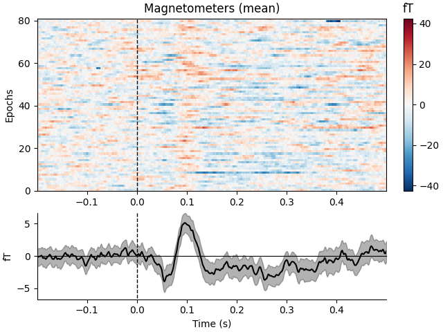
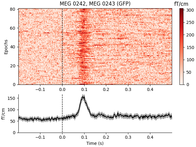
By default, the image map generated by plot_image will be
accompanied by a scalebar indicating the range of the colormap, and a time
series showing the average signal across epochs and a bootstrapped 95%
confidence band around the mean. plot_image is a highly
customizable method with many parameters, including customization of the
auxiliary colorbar and averaged time series subplots. See the docstrings of
plot_image and mne.viz.plot_compare_evokeds (which is
used to plot the average time series) for full details. Here we’ll show the
mean across magnetometers for all epochs with an auditory stimulus:
epochs["auditory"].plot_image(picks="mag", combine="mean")
Not setting metadata
81 matching events found
No baseline correction applied
0 projection items activated
combining channels using "mean"
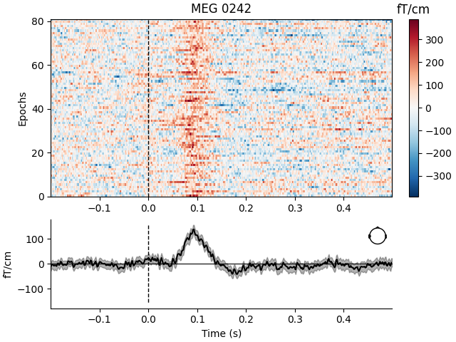
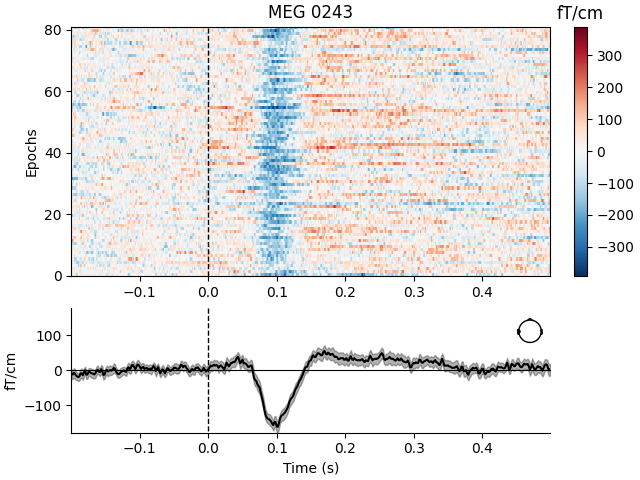
To plot image maps for individual sensors or a small group of sensors, use
the picks parameter. Passing combine=None (the default) will yield
separate plots for each sensor in picks; passing combine='gfp' will
plot the global field power (useful for combining sensors that respond with
opposite polarity).
Not setting metadata
81 matching events found
No baseline correction applied
0 projection items activated
Not setting metadata
81 matching events found
No baseline correction applied
0 projection items activated
Not setting metadata
81 matching events found
No baseline correction applied
0 projection items activated
combining channels using RMS (grad channels)
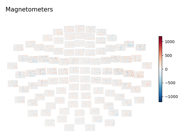
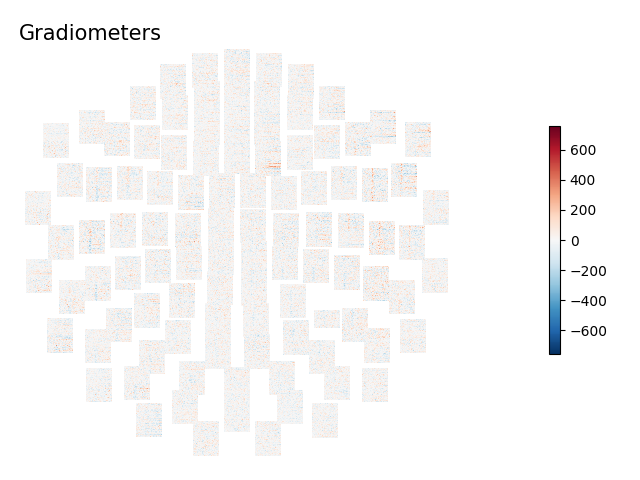
To plot an image map for all sensors, use
plot_topo_image, which is optimized for plotting a large
number of image maps simultaneously, and (in interactive sessions) allows you
to click on each small image map to pop open a separate figure with the
full-sized image plot (as if you had called plot_image on
just that sensor). At the small scale shown in this tutorial it’s hard to see
much useful detail in these plots; it’s often best when plotting
interactively to maximize the topo image plots to fullscreen. The default is
a figure with black background, so here we specify a white background and
black foreground text. By default plot_topo_image will
show magnetometers and gradiometers on the same plot (and hence not show a
colorbar, since the sensors are on different scales) so we’ll also pass a
Layout restricting each plot to one channel type.
First, however, we’ll also drop any epochs that have unusually high signal
levels, because they can cause the colormap limits to be too extreme and
therefore mask smaller signal fluctuations of interest.
reject_criteria = dict(
    mag=3000e-15,  # 3000 fT
    grad=3000e-13,  # 3000 fT/cm
    eeg=150e-6,
)  # 150 µV
epochs.drop_bad(reject=reject_criteria)

for ch_type, title in dict(mag="Magnetometers", grad="Gradiometers").items():
    layout = mne.channels.find_layout(epochs.info, ch_type=ch_type)
    epochs["auditory/left"].plot_topo_image(
        layout=layout, fig_facecolor="w", font_color="k", title=title
    )
    Rejecting  epoch based on EEG : ['EEG 001', 'EEG 002', 'EEG 003', 'EEG 004', 'EEG 005', 'EEG 006', 'EEG 007', 'EEG 015', 'EEG 016', 'EEG 023', 'EEG 039', 'EEG 041', 'EEG 044', 'EEG 045', 'EEG 046', 'EEG 047', 'EEG 048', 'EEG 049', 'EEG 050', 'EEG 051', 'EEG 052', 'EEG 054', 'EEG 055', 'EEG 056', 'EEG 057', 'EEG 058', 'EEG 059']
    Rejecting  epoch based on EEG : ['EEG 001', 'EEG 002', 'EEG 003', 'EEG 007', 'EEG 048', 'EEG 055']
    Rejecting  epoch based on EEG : ['EEG 007']
    Rejecting  epoch based on EEG : ['EEG 003', 'EEG 007']
    Rejecting  epoch based on MAG : ['MEG 1711']
    Rejecting  epoch based on EEG : ['EEG 001', 'EEG 002', 'EEG 003', 'EEG 007']
    Rejecting  epoch based on EEG : ['EEG 001', 'EEG 002', 'EEG 007']
    Rejecting  epoch based on MAG : ['MEG 1711']
8 bad epochs dropped
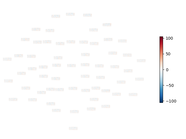
To plot image maps for all EEG sensors, pass an EEG layout as the layout
parameter of plot_topo_image. Note also here the use of
the sigma parameter, which smooths each image map along the vertical
dimension (across epochs) which can make it easier to see patterns across the
small image maps (by smearing noisy epochs onto their neighbors, while
reinforcing parts of the image where adjacent epochs are similar). However,
sigma can also disguise epochs that have persistent extreme values and
maybe should have been excluded, so it should be used with caution.
Total running time of the script: (0 minutes 31.718 seconds)