Note
Go to the end to download the full example code.
Compute source power estimate by projecting the covariance with MNE#
We can apply the MNE inverse operator to a covariance matrix to obtain an estimate of source power. This is computationally more efficient than first estimating the source timecourses and then computing their power. This code is based on the code from [1] and has been useful to correct for individual field spread using source localization in the context of predictive modeling.
References#
# Author: Denis A. Engemann <denis-alexander.engemann@inria.fr>
#         Luke Bloy <luke.bloy@gmail.com>
#
# License: BSD-3-Clause
# Copyright the MNE-Python contributors.
import numpy as np

import mne
from mne.datasets import sample
from mne.minimum_norm import apply_inverse_cov, make_inverse_operator

data_path = sample.data_path()
subjects_dir = data_path / "subjects"
meg_path = data_path / "MEG" / "sample"
raw_fname = meg_path / "sample_audvis_filt-0-40_raw.fif"
raw = mne.io.read_raw_fif(raw_fname)
Opening raw data file /home/circleci/mne_data/MNE-sample-data/MEG/sample/sample_audvis_filt-0-40_raw.fif...
    Read a total of 4 projection items:
        PCA-v1 (1 x 10²)  idle
        PCA-v2 (1 x 10²)  idle
        PCA-v3 (1 x 10²)  idle
        Average EEG reference (1 x 60)  idle
    Range : 6450 ... 48149 =     42.956 ...   320.665 secs
Ready.
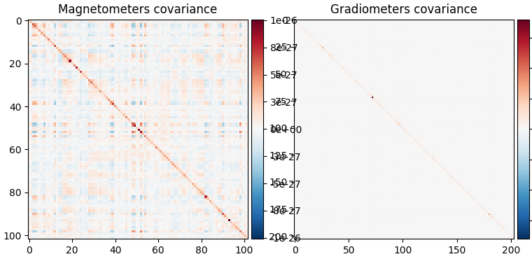
Compute empty-room covariance#
First we compute an empty-room covariance, which captures noise from the sensors and environment.
raw_empty_room_fname = data_path / "MEG" / "sample" / "ernoise_raw.fif"
raw_empty_room = mne.io.read_raw_fif(raw_empty_room_fname)
raw_empty_room.crop(0, 30)  # cropped just for speed
raw_empty_room.info["bads"] = ["MEG 2443"]
raw_empty_room.add_proj(raw.info["projs"])
noise_cov = mne.compute_raw_covariance(raw_empty_room, method="shrunk")
del raw_empty_room
Opening raw data file /home/circleci/mne_data/MNE-sample-data/MEG/sample/ernoise_raw.fif...
Isotrak not found
    Read a total of 3 projection items:
        PCA-v1 (1 x 10²)  idle
        PCA-v2 (1 x 10²)  idle
        PCA-v3 (1 x 10²)  idle
    Range : 19800 ... 85867 =     32.966 ...   142.965 secs
Ready.
4 projection items deactivated
Using up to 150 segments
Loading data for 150 events and 120 original time points ...
0 bad epochs dropped
    Created an SSP operator (subspace dimension = 3)
    Setting small MEG eigenvalues to zero (without PCA)
Reducing data rank from 305 -> 302
Estimating covariance using SHRUNK
Done.
Number of samples used : 18000
[done]
Epoch the data#
raw.pick(["meg", "stim", "eog"]).load_data().filter(4, 12)
raw.info["bads"] = ["MEG 2443"]
events = mne.find_events(raw, stim_channel="STI 014")
event_id = dict(aud_l=1, aud_r=2, vis_l=3, vis_r=4)
tmin, tmax = -0.2, 0.5
baseline = (None, 0)  # means from the first instant to t = 0
reject = dict(grad=4000e-13, mag=4e-12, eog=150e-6)
epochs = mne.Epochs(
    raw,
    events,
    event_id,
    tmin,
    tmax,
    proj=True,
    picks=("meg", "eog"),
    baseline=None,
    reject=reject,
    preload=True,
    decim=5,
    verbose="error",
)
del raw
Reading 0 ... 41699  =      0.000 ...   277.709 secs...
Filtering raw data in 1 contiguous segment
Setting up band-pass filter from 4 - 12 Hz

FIR filter parameters
---------------------
Designing a one-pass, zero-phase, non-causal bandpass filter:
- Windowed time-domain design (firwin) method
- Hamming window with 0.0194 passband ripple and 53 dB stopband attenuation
- Lower passband edge: 4.00
- Lower transition bandwidth: 2.00 Hz (-6 dB cutoff frequency: 3.00 Hz)
- Upper passband edge: 12.00 Hz
- Upper transition bandwidth: 3.00 Hz (-6 dB cutoff frequency: 13.50 Hz)
- Filter length: 249 samples (1.658 s)

Finding events on: STI 014
319 events found on stim channel STI 014
Event IDs: [ 1  2  3  4  5 32]
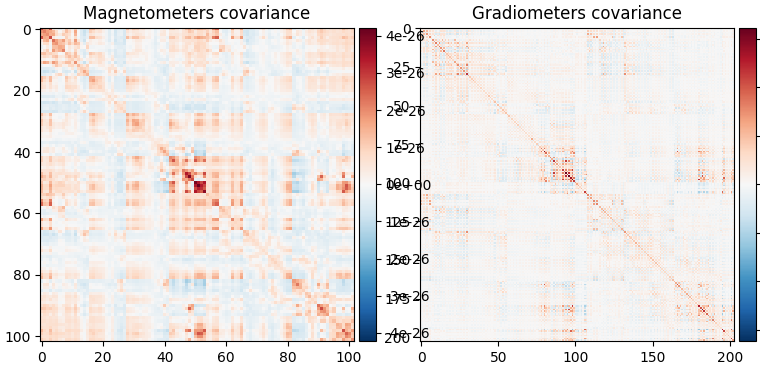
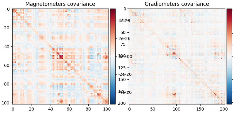
Compute and plot covariances#
In addition to the empty-room covariance above, we compute two additional covariances:
Baseline covariance, which captures signals not of interest in our analysis (e.g., sensor noise, environmental noise, physiological artifacts, and also resting-state-like brain activity / “noise”).
Data covariance, which captures our activation of interest (in addition to noise sources).
base_cov = mne.compute_covariance(
    epochs, tmin=-0.2, tmax=0, method="shrunk", verbose=True
)
data_cov = mne.compute_covariance(
    epochs, tmin=0.0, tmax=0.2, method="shrunk", verbose=True
)

fig_noise_cov = mne.viz.plot_cov(noise_cov, epochs.info, show_svd=False)
fig_base_cov = mne.viz.plot_cov(base_cov, epochs.info, show_svd=False)
fig_data_cov = mne.viz.plot_cov(data_cov, epochs.info, show_svd=False)
    Created an SSP operator (subspace dimension = 3)
    Setting small MEG eigenvalues to zero (without PCA)
Reducing data rank from 305 -> 302
Estimating covariance using SHRUNK
Done.
Number of samples used : 1680
[done]
    Created an SSP operator (subspace dimension = 3)
    Setting small MEG eigenvalues to zero (without PCA)
Reducing data rank from 305 -> 302
Estimating covariance using SHRUNK
Done.
Number of samples used : 1680
[done]
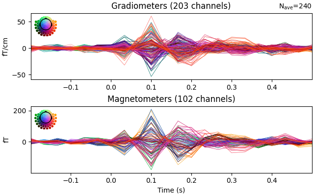
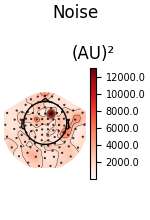
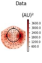
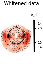
We can also look at the covariances using topomaps, here we just show the baseline and data covariances, followed by the data covariance whitened by the baseline covariance:
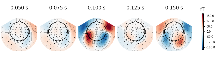
evoked = epochs.average().pick("meg")
evoked.drop_channels(evoked.info["bads"])
evoked.plot(time_unit="s")
evoked.plot_topomap(times=np.linspace(0.05, 0.15, 5), ch_type="mag")

loop = {
    "Noise": (noise_cov, dict()),
    "Data": (data_cov, dict()),
    "Whitened data": (data_cov, dict(noise_cov=noise_cov)),
}
for title, (_cov, _kw) in loop.items():
    fig = _cov.plot_topomap(evoked.info, "grad", **_kw)
    fig.suptitle(title)
    Created an SSP operator (subspace dimension = 3)
Computing rank from covariance with rank=None
    Using tolerance 1.4e-13 (2.2e-16 eps * 305 dim * 2.1  max singular value)
    Estimated rank (mag + grad): 302
    MEG: rank 302 computed from 305 data channels with 3 projectors
    Setting small MEG eigenvalues to zero (without PCA)
    Created the whitener using a noise covariance matrix with rank 302 (3 small eigenvalues omitted)
Apply inverse operator to covariance#
Finally, we can construct an inverse using the empty-room noise covariance:
# Read the forward solution and compute the inverse operator
fname_fwd = meg_path / "sample_audvis-meg-oct-6-fwd.fif"
fwd = mne.read_forward_solution(fname_fwd)
# make an MEG inverse operator
info = evoked.info
inverse_operator = make_inverse_operator(info, fwd, noise_cov, loose=0.2, depth=0.8)
Reading forward solution from /home/circleci/mne_data/MNE-sample-data/MEG/sample/sample_audvis-meg-oct-6-fwd.fif...
    Reading a source space...
    Computing patch statistics...
    Patch information added...
    Distance information added...
    [done]
    Reading a source space...
    Computing patch statistics...
    Patch information added...
    Distance information added...
    [done]
    2 source spaces read
    Desired named matrix (kind = 3523 (FIFF_MNE_FORWARD_SOLUTION_GRAD)) not available
    Read MEG forward solution (7498 sources, 306 channels, free orientations)
    Source spaces transformed to the forward solution coordinate frame
Converting forward solution to surface orientation
    Average patch normals will be employed in the rotation to the local surface coordinates....
    Converting to surface-based source orientations...
    [done]
Computing inverse operator with 305 channels.
    305 out of 306 channels remain after picking
Selected 305 channels
Creating the depth weighting matrix...
    203 planar channels
    limit = 7265/7498 = 10.037795
    scale = 2.52065e-08 exp = 0.8
Applying loose dipole orientations to surface source spaces: 0.2
Whitening the forward solution.
    Created an SSP operator (subspace dimension = 3)
Computing rank from covariance with rank=None
    Using tolerance 1.4e-13 (2.2e-16 eps * 305 dim * 2.1  max singular value)
    Estimated rank (mag + grad): 302
    MEG: rank 302 computed from 305 data channels with 3 projectors
    Setting small MEG eigenvalues to zero (without PCA)
Creating the source covariance matrix
Adjusting source covariance matrix.
Computing SVD of whitened and weighted lead field matrix.
    largest singular value = 6.411
    scaling factor to adjust the trace = 5.63162e+19 (nchan = 305 nzero = 3)
Project our data and baseline covariance to source space:
stc_data = apply_inverse_cov(
    data_cov,
    evoked.info,
    inverse_operator,
    nave=len(epochs),
    method="dSPM",
    verbose=True,
)
stc_base = apply_inverse_cov(
    base_cov,
    evoked.info,
    inverse_operator,
    nave=len(epochs),
    method="dSPM",
    verbose=True,
)
Preparing the inverse operator for use...
    Scaled noise and source covariance from nave = 1 to nave = 240
    Created the regularized inverter
    Created an SSP operator (subspace dimension = 3)
    Created the whitener using a noise covariance matrix with rank 302 (3 small eigenvalues omitted)
    Computing noise-normalization factors (dSPM)...
[done]
Applying inverse operator to "cov"...
    Picked 305 channels from the data
    Computing inverse...
    Eigenleads need to be weighted ...
    Computing residual...
    Explained  37.1% variance
    dSPM...
    Combining the current components...
[done]
And visualize power is relative to the baseline:
stc_data /= stc_base
brain = stc_data.plot(
    subject="sample",
    subjects_dir=subjects_dir,
    clim=dict(kind="percent", lims=(50, 90, 98)),
    smoothing_steps=7,
)
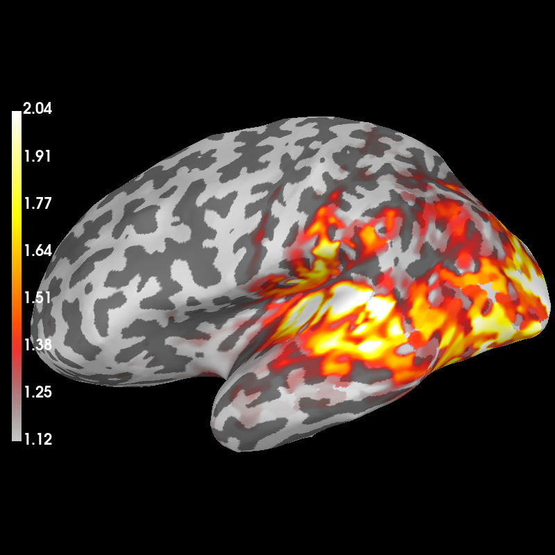
Using control points [1.11813641 1.45873675 2.03828176]
Total running time of the script: (0 minutes 34.917 seconds)