Extracting the time series of activations in a label

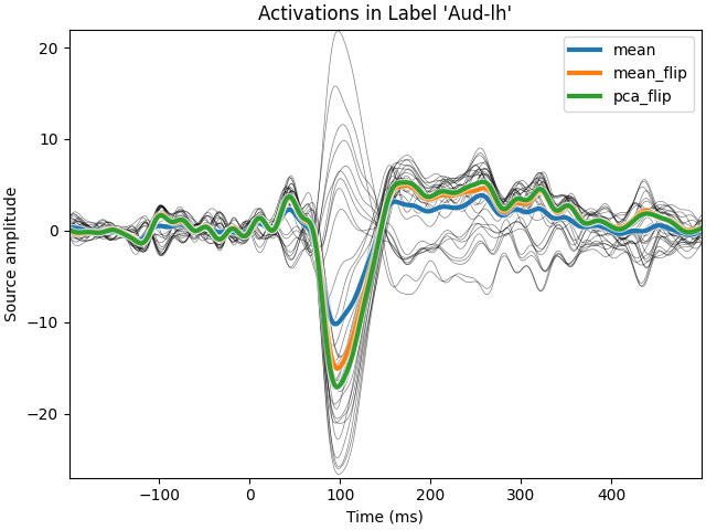
We first apply a dSPM inverse operator to get signed activations in a label (with positive and negative values) and we then compare different strategies to average the times series in a label. We compare a simple average, with an averaging using the dipoles normal (flip mode) and then a PCA, also using a sign flip.

# Authors: Alexandre Gramfort <alexandre.gramfort@inria.fr>
#          Eric Larson <larson.eric.d@gmail.com>
#
# License: BSD-3-Clause
# Copyright the MNE-Python contributors.

import matplotlib.patheffects as path_effects
import matplotlib.pyplot as plt

import mne
from mne.datasets import sample
from mne.minimum_norm import apply_inverse, read_inverse_operator

print(__doc__)

data_path = sample.data_path()
label = "Aud-lh"
meg_path = data_path / "MEG" / "sample"
label_fname = meg_path / "labels" / f"{label}.label"
fname_inv = meg_path / "sample_audvis-meg-oct-6-meg-inv.fif"
fname_evoked = meg_path / "sample_audvis-ave.fif"

snr = 3.0
lambda2 = 1.0 / snr**2
method = "dSPM"  # use dSPM method (could also be MNE or sLORETA)

# Load data
evoked = mne.read_evokeds(fname_evoked, condition=0, baseline=(None, 0))
inverse_operator = read_inverse_operator(fname_inv)
src = inverse_operator["src"]

Reading /home/circleci/mne_data/MNE-sample-data/MEG/sample/sample_audvis-ave.fif ...
    Read a total of 4 projection items:
        PCA-v1 (1 x 102) active
        PCA-v2 (1 x 102) active
        PCA-v3 (1 x 102) active
        Average EEG reference (1 x 60) active
    Found the data of interest:
        t =    -199.80 ...     499.49 ms (Left Auditory)
        0 CTF compensation matrices available
        nave = 55 - aspect type = 100
Projections have already been applied. Setting proj attribute to True.
Applying baseline correction (mode: mean)
Reading inverse operator decomposition from /home/circleci/mne_data/MNE-sample-data/MEG/sample/sample_audvis-meg-oct-6-meg-inv.fif...
    Reading inverse operator info...
    [done]
    Reading inverse operator decomposition...
    [done]
    305 x 305 full covariance (kind = 1) found.
    Read a total of 4 projection items:
        PCA-v1 (1 x 102) active
        PCA-v2 (1 x 102) active
        PCA-v3 (1 x 102) active
        Average EEG reference (1 x 60) active
    Noise covariance matrix read.
    22494 x 22494 diagonal covariance (kind = 2) found.
    Source covariance matrix read.
    22494 x 22494 diagonal covariance (kind = 6) found.
    Orientation priors read.
    22494 x 22494 diagonal covariance (kind = 5) found.
    Depth priors read.
    Did not find the desired covariance matrix (kind = 3)
    Reading a source space...
    Computing patch statistics...
    Patch information added...
    Distance information added...
    [done]
    Reading a source space...
    Computing patch statistics...
    Patch information added...
    Distance information added...
    [done]
    2 source spaces read
    Read a total of 4 projection items:
        PCA-v1 (1 x 102) active
        PCA-v2 (1 x 102) active
        PCA-v3 (1 x 102) active
        Average EEG reference (1 x 60) active
    Source spaces transformed to the inverse solution coordinate frame

Compute inverse solution

pick_ori = "normal"  # Get signed values to see the effect of sign flip
stc = apply_inverse(evoked, inverse_operator, lambda2, method, pick_ori=pick_ori)

label = mne.read_label(label_fname)

stc_label = stc.in_label(label)
modes = ("mean", "mean_flip", "pca_flip")
tcs = dict()
for mode in modes:
    tcs[mode] = stc.extract_label_time_course(label, src, mode=mode)
print("Number of vertices : %d" % len(stc_label.data))

Preparing the inverse operator for use...
    Scaled noise and source covariance from nave = 1 to nave = 55
    Created the regularized inverter
    Created an SSP operator (subspace dimension = 3)
    Created the whitener using a noise covariance matrix with rank 302 (3 small eigenvalues omitted)
    Computing noise-normalization factors (dSPM)...
[done]
Applying inverse operator to "Left Auditory"...
    Picked 305 channels from the data
    Computing inverse...
    Eigenleads need to be weighted ...
    Computing residual...
    Explained  59.4% variance
    dSPM...
[done]
Extracting time courses for 1 labels (mode: mean)
Extracting time courses for 1 labels (mode: mean_flip)
Extracting time courses for 1 labels (mode: pca_flip)
Number of vertices : 33

View source activations

fig, ax = plt.subplots(1, layout="constrained")
t = 1e3 * stc_label.times
ax.plot(t, stc_label.data.T, "k", linewidth=0.5, alpha=0.5)
pe = [
    path_effects.Stroke(linewidth=5, foreground="w", alpha=0.5),
    path_effects.Normal(),
]
for mode, tc in tcs.items():
    ax.plot(t, tc[0], linewidth=3, label=str(mode), path_effects=pe)
xlim = t[[0, -1]]
ylim = [-27, 22]
ax.legend(loc="upper right")
ax.set(
    xlabel="Time (ms)",
    ylabel="Source amplitude",
    title="Activations in Label %r" % (label.name),
    xlim=xlim,
    ylim=ylim,
)

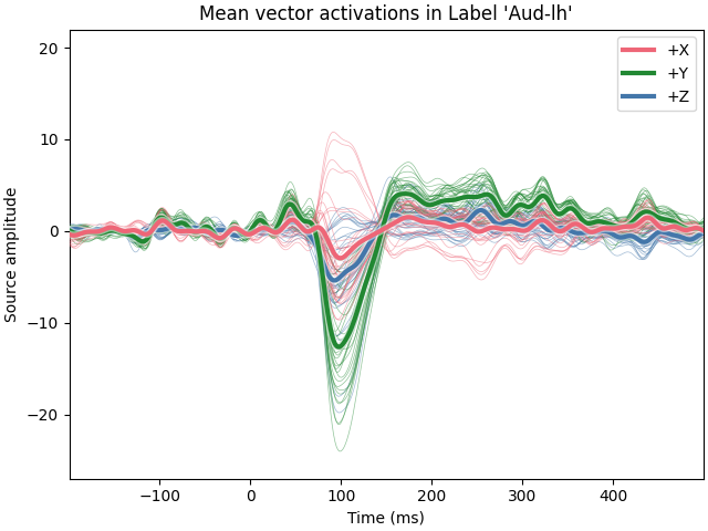
Using vector solutions

It’s also possible to compute label time courses for a mne.VectorSourceEstimate, but only with mode='mean'.

pick_ori = "vector"
stc_vec = apply_inverse(evoked, inverse_operator, lambda2, method, pick_ori=pick_ori)
data = stc_vec.extract_label_time_course(label, src)
fig, ax = plt.subplots(1, layout="constrained")
stc_vec_label = stc_vec.in_label(label)
colors = ["#EE6677", "#228833", "#4477AA"]
for ii, name in enumerate("XYZ"):
    color = colors[ii]
    ax.plot(
        t, stc_vec_label.data[:, ii].T, color=color, lw=0.5, alpha=0.5, zorder=5 - ii
    )
    ax.plot(
        t,
        data[0, ii],
        lw=3,
        color=color,
        label="+" + name,
        zorder=8 - ii,
        path_effects=pe,
    )
ax.legend(loc="upper right")
ax.set(
    xlabel="Time (ms)",
    ylabel="Source amplitude",
    title=f"Mean vector activations in Label {label.name!r}",
    xlim=xlim,
    ylim=ylim,
)

Preparing the inverse operator for use...
    Scaled noise and source covariance from nave = 1 to nave = 55
    Created the regularized inverter
    Created an SSP operator (subspace dimension = 3)
    Created the whitener using a noise covariance matrix with rank 302 (3 small eigenvalues omitted)
    Computing noise-normalization factors (dSPM)...
[done]
Applying inverse operator to "Left Auditory"...
    Picked 305 channels from the data
    Computing inverse...
    Eigenleads need to be weighted ...
    Computing residual...
    Explained  59.4% variance
    dSPM...
[done]
Extracting time courses for 1 labels (mode: mean)

Estimated memory usage: 163 MB