Repairing artifacts with ICA

This tutorial covers the basics of independent components analysis (ICA) and shows how ICA can be used for artifact repair; an extended example illustrates repair of ocular and heartbeat artifacts. For conceptual background on ICA, see this scikit-learn tutorial.

We begin as always by importing the necessary Python modules and loading some example data. Because ICA can be computationally intense, we’ll also crop the data to 60 seconds; and to save ourselves from repeatedly typing mne.preprocessing we’ll directly import a few functions and classes from that submodule:

# Authors: The MNE-Python contributors.
# License: BSD-3-Clause
# Copyright the MNE-Python contributors.

import os

import mne
from mne.preprocessing import ICA, corrmap, create_ecg_epochs, create_eog_epochs

sample_data_folder = mne.datasets.sample.data_path()
sample_data_raw_file = os.path.join(
    sample_data_folder, "MEG", "sample", "sample_audvis_filt-0-40_raw.fif"
)
raw = mne.io.read_raw_fif(sample_data_raw_file)

# Here we'll crop to 60 seconds and drop gradiometer channels for speed
raw.crop(tmax=60.0).pick(picks=["mag", "eeg", "stim", "eog"])
raw.load_data()

Opening raw data file /home/circleci/mne_data/MNE-sample-data/MEG/sample/sample_audvis_filt-0-40_raw.fif...
    Read a total of 4 projection items:
        PCA-v1 (1 x 102)  idle
        PCA-v2 (1 x 102)  idle
        PCA-v3 (1 x 102)  idle
        Average EEG reference (1 x 60)  idle
    Range : 6450 ... 48149 =     42.956 ...   320.665 secs
Ready.
Reading 0 ... 9009  =      0.000 ...    59.999 secs...

	General
	Filename(s)	sample_audvis_filt-0-40_raw.fif
	MNE object type	Raw
	Measurement date	2002-12-03 at 19:01:10 UTC
	Participant	Unknown
	Experimenter	Unknown
	Acquisition
	Duration	00:00:60 (HH:MM:SS)
	Sampling frequency	150.15 Hz
	Time points	9,010
	Channels
	Magnetometers	102
	EEG	59 and 1 bad
	EOG	1
	Stimulus	9
	Head & sensor digitization	146 points
	Filters
	Highpass	0.10 Hz
	Lowpass	40.00 Hz
	Projections	PCA-v1 (off) PCA-v2 (off) PCA-v3 (off) Average EEG reference (off)

Note

Before applying ICA (or any artifact repair strategy), be sure to observe the artifacts in your data to make sure you choose the right repair tool. Sometimes the right tool is no tool at all — if the artifacts are small enough you may not even need to repair them to get good analysis results. See Overview of artifact detection for guidance on detecting and visualizing various types of artifact.

What is ICA?

Independent components analysis (ICA) is a technique for estimating independent source signals from a set of recordings in which the source signals were mixed together in unknown ratios. A common example of this is the problem of blind source separation: with 3 musical instruments playing in the same room, and 3 microphones recording the performance (each picking up all 3 instruments, but at varying levels), can you somehow “unmix” the signals recorded by the 3 microphones so that you end up with a separate “recording” isolating the sound of each instrument?

It is not hard to see how this analogy applies to EEG/MEG analysis: there are many “microphones” (sensor channels) simultaneously recording many “instruments” (blinks, heartbeats, activity in different areas of the brain, muscular activity from jaw clenching or swallowing, etc). As long as these various source signals are statistically independent and non-gaussian, it is usually possible to separate the sources using ICA, and then re-construct the sensor signals after excluding the sources that are unwanted.

ICA in MNE-Python

ICA and dimensionality reduction

If you want to perform ICA with no dimensionality reduction (other than the number of Independent Components (ICs) given in n_components, and any subsequent exclusion of ICs you specify in ICA.exclude), simply pass n_components.

However, if you do want to reduce dimensionality, consider this example: if you have 300 sensor channels and you set n_components=50 during instantiation and pass n_pca_components=None to apply, then the the first 50 PCs are sent to the ICA algorithm (yielding 50 ICs), and during reconstruction apply will use the 50 ICs plus PCs number 51-300 (the full PCA residual). If instead you specify n_pca_components=120 in apply, it will reconstruct using the 50 ICs plus the first 70 PCs in the PCA residual (numbers 51-120), thus discarding the smallest 180 components.

If you have previously been using EEGLAB’s runica() and are looking for the equivalent of its 'pca', n option to reduce dimensionality, set n_components=n during initialization and pass n_pca_components=n to apply.

MNE-Python implements three different ICA algorithms: fastica (the default), picard, and infomax. FastICA and Infomax are both in fairly widespread use; Picard is a newer (2017) algorithm that is expected to converge faster than FastICA and Infomax, and is more robust than other algorithms in cases where the sources are not completely independent, which typically happens with real EEG/MEG data. See [1] for more information.

The ICA interface in MNE-Python is similar to the interface in scikit-learn: some general parameters are specified when creating an ICA object, then the ICA object is fit to the data using its fit method. The results of the fitting are added to the ICA object as attributes that end in an underscore (_), such as ica.mixing_matrix_ and ica.unmixing_matrix_. After fitting, the ICA component(s) that you want to remove must be chosen, and the ICA fit must then be applied to the Raw or Epochs object using the ICA object’s apply method.

As is typically done with ICA, the data are first scaled to unit variance and whitened using principal components analysis (PCA) before performing the ICA decomposition. This is a two-stage process:

1. To deal with different channel types having different units (e.g., Volts for EEG and Tesla for MEG), data must be pre-whitened. If noise_cov=None (default), all data of a given channel type is scaled by the standard deviation across all channels. If noise_cov is a Covariance, the channels are pre-whitened using the covariance.

2. The pre-whitened data are then decomposed using PCA.

From the resulting principal components (PCs), the first n_components are then passed to the ICA algorithm if n_components is an integer number. It can also be a float between 0 and 1, specifying the fraction of explained variance that the PCs should capture; the appropriate number of PCs (i.e., just as many PCs as are required to explain the given fraction of total variance) is then passed to the ICA.

After visualizing the Independent Components (ICs) and excluding any that capture artifacts you want to repair, the sensor signal can be reconstructed using the ICA object’s apply method. By default, signal reconstruction uses all of the ICs (less any ICs listed in ICA.exclude) plus all of the PCs that were not included in the ICA decomposition (i.e., the “PCA residual”). If you want to reduce the number of components used at the reconstruction stage, it is controlled by the n_pca_components parameter (which will in turn reduce the rank of your data; by default n_pca_components=None resulting in no additional dimensionality reduction). The fitting and reconstruction procedures and the parameters that control dimensionality at various stages are summarized in the diagram below:

See the Notes section of the ICA documentation for further details. Next we’ll walk through an extended example that illustrates each of these steps in greater detail.

Example: EOG and ECG artifact repair

Visualizing the artifacts

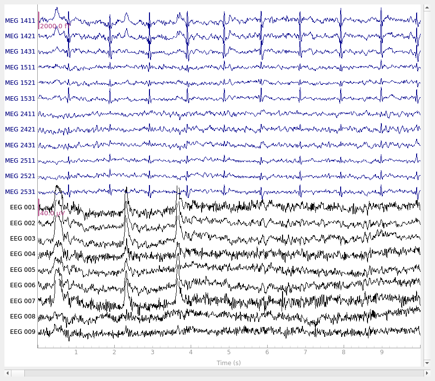
Let’s begin by visualizing the artifacts that we want to repair. In this dataset they are big enough to see easily in the raw data:

# pick some channels that clearly show heartbeats and blinks
regexp = r"(MEG [12][45][123]1|EEG 00.)"
artifact_picks = mne.pick_channels_regexp(raw.ch_names, regexp=regexp)
raw.plot(order=artifact_picks, n_channels=len(artifact_picks), show_scrollbars=False)

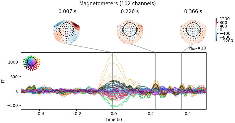
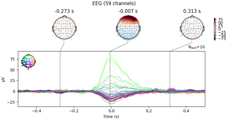
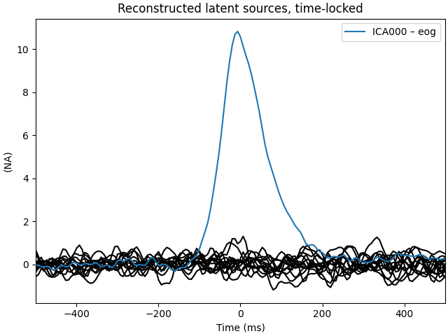
We can get a summary of how the ocular artifact manifests across each channel type using create_eog_epochs like we did in the Overview of artifact detection tutorial:

eog_evoked = create_eog_epochs(raw).average()
eog_evoked.apply_baseline(baseline=(None, -0.2))
eog_evoked.plot_joint()

• 
• 

Using EOG channel: EOG 061
EOG channel index for this subject is: [171]
Filtering the data to remove DC offset to help distinguish blinks from saccades
Selecting channel EOG 061 for blink detection
Setting up band-pass filter from 1 - 10 Hz

FIR filter parameters
---------------------
Designing a two-pass forward and reverse, zero-phase, non-causal bandpass filter:
- Windowed frequency-domain design (firwin2) method
- Hann window
- Lower passband edge: 1.00
- Lower transition bandwidth: 0.50 Hz (-12 dB cutoff frequency: 0.75 Hz)
- Upper passband edge: 10.00 Hz
- Upper transition bandwidth: 0.50 Hz (-12 dB cutoff frequency: 10.25 Hz)
- Filter length: 1502 samples (10.003 s)

Now detecting blinks and generating corresponding events
Found 10 significant peaks
Number of EOG events detected: 10
Not setting metadata
10 matching events found
No baseline correction applied
Created an SSP operator (subspace dimension = 4)
Using data from preloaded Raw for 10 events and 151 original time points ...
0 bad epochs dropped
Applying baseline correction (mode: mean)
Created an SSP operator (subspace dimension = 4)
4 projection items activated
SSP projectors applied...

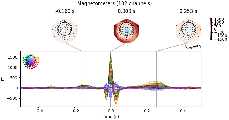
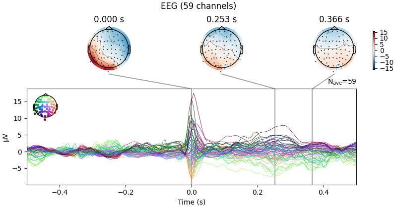
Now we’ll do the same for the heartbeat artifacts, using create_ecg_epochs:

ecg_evoked = create_ecg_epochs(raw).average()
ecg_evoked.apply_baseline(baseline=(None, -0.2))
ecg_evoked.plot_joint()

• 
• 

Reconstructing ECG signal from Magnetometers
Setting up band-pass filter from 8 - 16 Hz

FIR filter parameters
---------------------
Designing a two-pass forward and reverse, zero-phase, non-causal bandpass filter:
- Windowed frequency-domain design (firwin2) method
- Hann window
- Lower passband edge: 8.00
- Lower transition bandwidth: 0.50 Hz (-12 dB cutoff frequency: 7.75 Hz)
- Upper passband edge: 16.00 Hz
- Upper transition bandwidth: 0.50 Hz (-12 dB cutoff frequency: 16.25 Hz)
- Filter length: 1502 samples (10.003 s)

Number of ECG events detected : 59 (average pulse 58.99492412402019 / min.)
Not setting metadata
59 matching events found
No baseline correction applied
Created an SSP operator (subspace dimension = 4)
Using data from preloaded Raw for 59 events and 151 original time points ...
0 bad epochs dropped
Applying baseline correction (mode: mean)
Created an SSP operator (subspace dimension = 4)
4 projection items activated
SSP projectors applied...

Filtering to remove slow drifts

Before we run the ICA, an important step is filtering the data to remove low-frequency drifts, which can negatively affect the quality of the ICA fit. The slow drifts are problematic because they reduce the independence of the assumed-to-be-independent sources (e.g., during a slow upward drift, the neural, heartbeat, blink, and other muscular sources will all tend to have higher values), making it harder for the algorithm to find an accurate solution. A high-pass filter with 1 Hz cutoff frequency is recommended. However, because filtering is a linear operation, the ICA solution found from the filtered signal can be applied to the unfiltered signal (see [2] for more information), so we’ll keep a copy of the unfiltered Raw object around so we can apply the ICA solution to it later.

filt_raw = raw.copy().filter(l_freq=1.0, h_freq=None)

Filtering raw data in 1 contiguous segment
Setting up high-pass filter at 1 Hz

FIR filter parameters
---------------------
Designing a one-pass, zero-phase, non-causal highpass filter:
- Windowed time-domain design (firwin) method
- Hamming window with 0.0194 passband ripple and 53 dB stopband attenuation
- Lower passband edge: 1.00
- Lower transition bandwidth: 1.00 Hz (-6 dB cutoff frequency: 0.50 Hz)
- Filter length: 497 samples (3.310 s)

[Parallel(n_jobs=1)]: Done  17 tasks      | elapsed:    0.0s
[Parallel(n_jobs=1)]: Done  71 tasks      | elapsed:    0.0s
[Parallel(n_jobs=1)]: Done 161 tasks      | elapsed:    0.1s

Fitting ICA

Ignoring the time domain

The ICA algorithms implemented in MNE-Python find patterns across channels, but ignore the time domain. This means you can compute ICA on discontinuous Epochs or Evoked objects (not just continuous Raw objects), or only use every Nth sample by passing the decim parameter to ICA.fit().

Now we’re ready to set up and fit the ICA. Since we know (from observing our raw data) that the EOG and ECG artifacts are fairly strong, we would expect those artifacts to be captured in the first few dimensions of the PCA decomposition that happens before the ICA. Therefore, we probably don’t need a huge number of components to do a good job of isolating our artifacts (though it is usually preferable to include more components for a more accurate solution). As a first guess, we’ll run ICA with n_components=15 (use only the first 15 PCA components to compute the ICA decomposition) — a very small number given that our data has over 300 channels, but with the advantage that it will run quickly and we will able to tell easily whether it worked or not (because we already know what the EOG / ECG artifacts should look like).

ICA fitting is not deterministic (e.g., the components may get a sign flip on different runs, or may not always be returned in the same order), so we’ll also specify a random seed so that we get identical results each time this tutorial is built by our web servers.

Warning

Epochs used for fitting ICA should not be baseline-corrected. Because cleaning the data via ICA may introduce DC offsets, we suggest to baseline correct your data after cleaning (and not before), should you require baseline correction.

ica = ICA(n_components=15, max_iter="auto", random_state=97)
ica.fit(filt_raw)
ica

Fitting ICA to data using 161 channels (please be patient, this may take a while)
Selecting by number: 15 components
Fitting ICA took 0.4s.

Method	fastica
Fit parameters	algorithm=parallel fun=logcosh fun_args=None max_iter=1000
Fit	22 iterations on raw data (9010 samples)
ICA components	15
Available PCA components	161
Channel types	mag, eeg
ICA components marked for exclusion	—

Some optional parameters that we could have passed to the fit method include decim (to use only every Nth sample in computing the ICs, which can yield a considerable speed-up) and reject (for providing a rejection dictionary for maximum acceptable peak-to-peak amplitudes for each channel type, just like we used when creating epoched data in the Overview of MEG/EEG analysis with MNE-Python tutorial).

Looking at the ICA solution

Now we can examine the ICs to see what they captured.

Using get_explained_variance_ratio(), we can retrieve the fraction of variance in the original data that is explained by our ICA components in the form of a dictionary:

explained_var_ratio = ica.get_explained_variance_ratio(filt_raw)
for channel_type, ratio in explained_var_ratio.items():
    print(f"Fraction of {channel_type} variance explained by all components: {ratio}")

Fraction of mag variance explained by all components: 0.9358001342790973
Fraction of eeg variance explained by all components: 0.7798689203334388

The values were calculated for all ICA components jointly, but separately for each channel type (here: magnetometers and EEG).

We can also explicitly request for which component(s) and channel type(s) to perform the computation:

explained_var_ratio = ica.get_explained_variance_ratio(
    filt_raw, components=[0], ch_type="eeg"
)
# This time, print as percentage.
ratio_percent = round(100 * explained_var_ratio["eeg"])
print(
    f"Fraction of variance in EEG signal explained by first component: "
    f"{ratio_percent}%"
)

Fraction of variance in EEG signal explained by first component: 33%

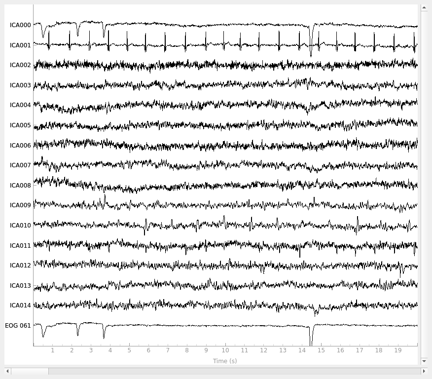
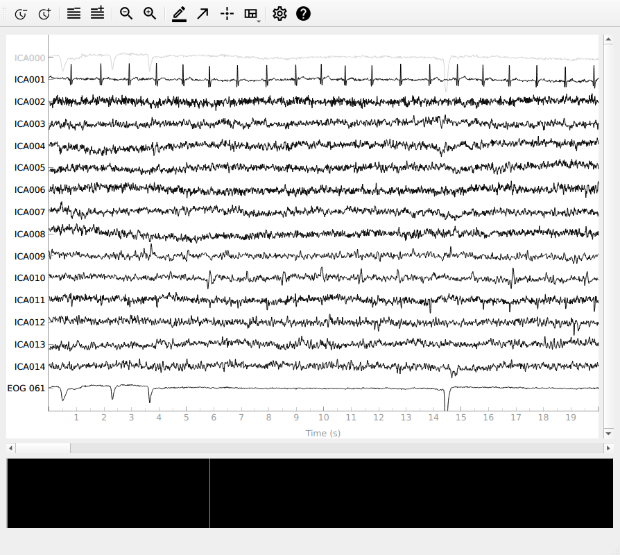
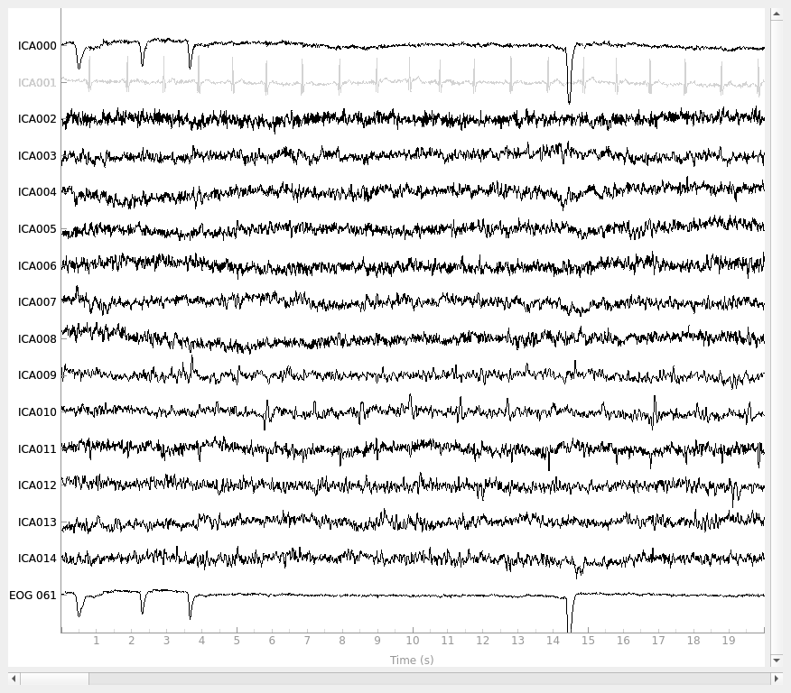
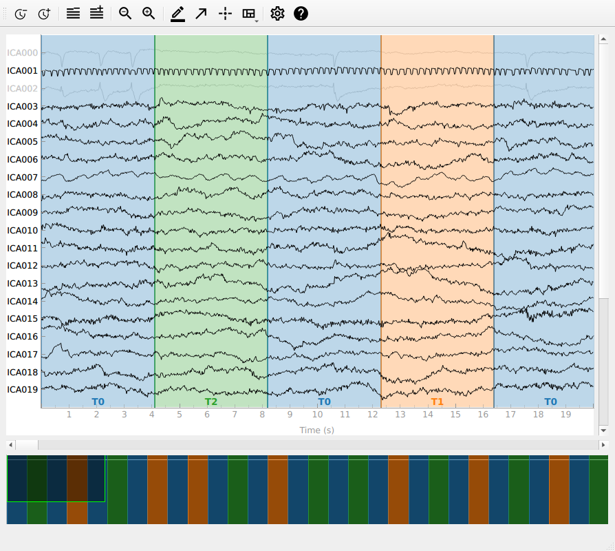
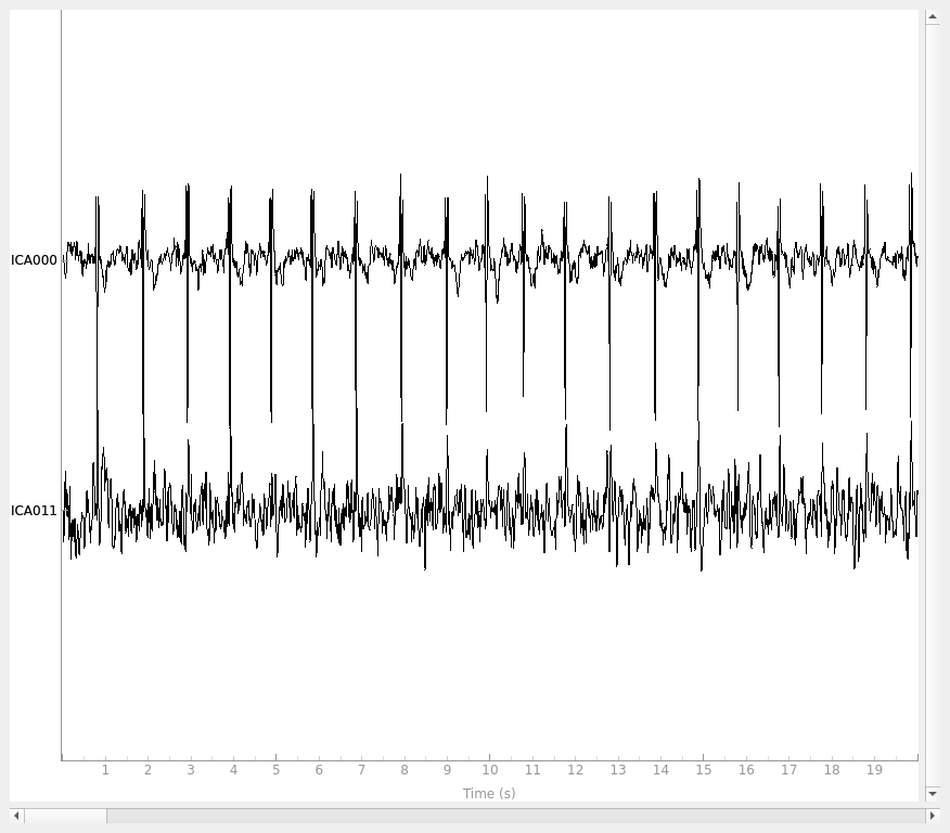
plot_sources will show the time series of the ICs. Note that in our call to plot_sources we can use the original, unfiltered Raw object. A helpful tip is that right clicking (or control + click with a trackpad) on the name of the component will bring up a plot of its properties. In this plot, you can also toggle the channel type in the topoplot (if you have multiple channel types) with ‘t’ and whether the spectrum is log-scaled or not with ‘l’.

raw.load_data()
ica.plot_sources(raw, show_scrollbars=False)

Creating RawArray with float64 data, n_channels=16, n_times=9010
    Range : 6450 ... 15459 =     42.956 ...   102.954 secs
Ready.

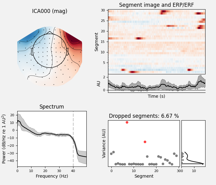
Here we can pretty clearly see that the first component (ICA000) captures the EOG signal quite well, and the second component (ICA001) looks a lot like a heartbeat (for more info on visually identifying Independent Components, this EEGLAB tutorial is a good resource). We can also visualize the scalp field distribution of each component using plot_components. These are interpolated based on the values in the ICA mixing matrix:

ica.plot_components()

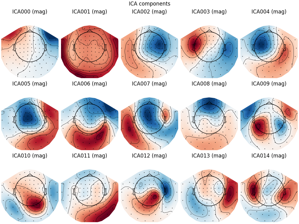
Note

plot_components (which plots the scalp field topographies for each component) has an optional inst parameter that takes an instance of Raw or Epochs. Passing inst makes the scalp topographies interactive: clicking one will bring up a diagnostic plot_properties window (see below) for that component.

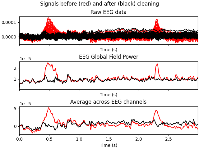
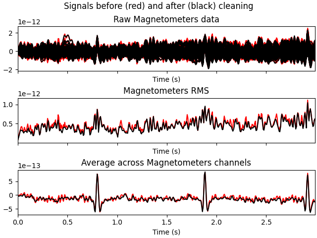
In the plots above it’s fairly obvious which ICs are capturing our EOG and ECG artifacts, but there are additional ways visualize them anyway just to be sure. First, we can plot an overlay of the original signal against the reconstructed signal with the artifactual ICs excluded, using plot_overlay:

# blinks
ica.plot_overlay(raw, exclude=[0], picks="eeg")
# heartbeats
ica.plot_overlay(raw, exclude=[1], picks="mag")

• 
• 

Applying ICA to Raw instance
    Transforming to ICA space (15 components)
    Zeroing out 1 ICA component
    Projecting back using 161 PCA components
Applying ICA to Raw instance
    Transforming to ICA space (15 components)
    Zeroing out 1 ICA component
    Projecting back using 161 PCA components

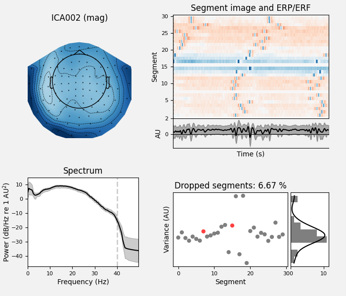
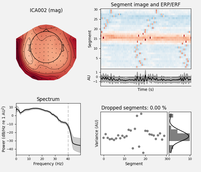
We can also plot some diagnostics of each IC using plot_properties:

ica.plot_properties(raw, picks=[0, 1])

• 
• 

    Using multitaper spectrum estimation with 7 DPSS windows
Not setting metadata
30 matching events found
No baseline correction applied
0 projection items activated
Not setting metadata
30 matching events found
No baseline correction applied
0 projection items activated

In the remaining sections, we’ll look at different ways of choosing which ICs to exclude prior to reconstructing the sensor signals.

Selecting ICA components manually

Once we’re certain which components we want to exclude, we can specify that manually by setting the ica.exclude attribute. Similar to marking bad channels, merely setting ica.exclude doesn’t do anything immediately (it just adds the excluded ICs to a list that will get used later when it’s needed). Once the exclusions have been set, ICA methods like plot_overlay will exclude those component(s) even if no exclude parameter is passed, and the list of excluded components will be preserved when using mne.preprocessing.ICA.save and mne.preprocessing.read_ica.

ica.exclude = [0, 1]  # indices chosen based on various plots above

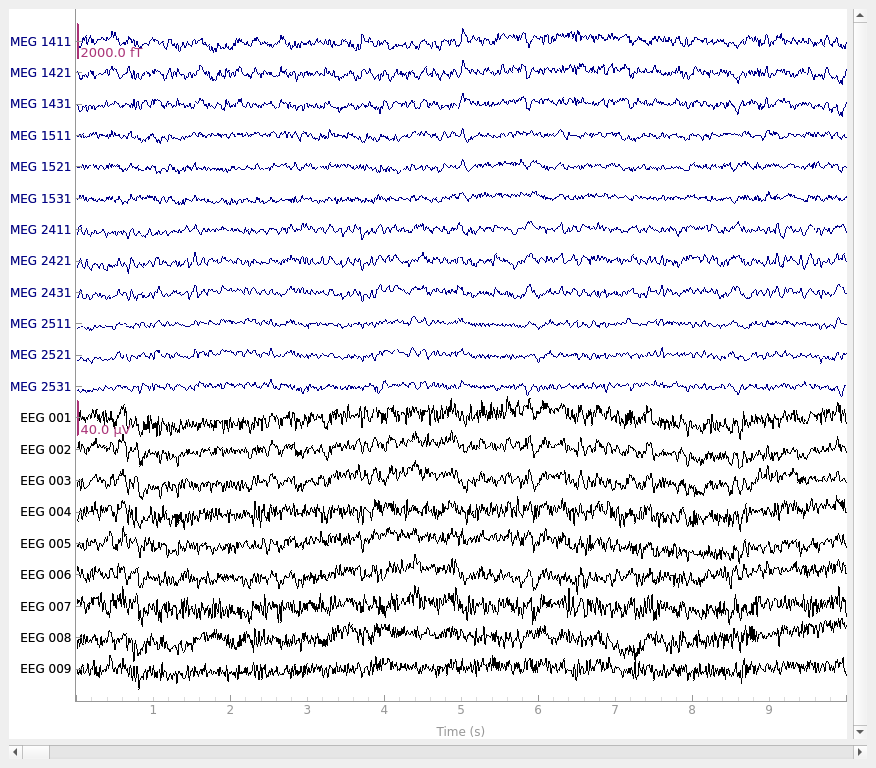
Now that the exclusions have been set, we can reconstruct the sensor signals with artifacts removed using the apply method (remember, we’re applying the ICA solution from the filtered data to the original unfiltered signal). Plotting the original raw data alongside the reconstructed data shows that the heartbeat and blink artifacts are repaired.

# ica.apply() changes the Raw object in-place, so let's make a copy first:
reconst_raw = raw.copy()
ica.apply(reconst_raw)

raw.plot(order=artifact_picks, n_channels=len(artifact_picks), show_scrollbars=False)
reconst_raw.plot(
    order=artifact_picks, n_channels=len(artifact_picks), show_scrollbars=False
)
del reconst_raw

• 
• 

Applying ICA to Raw instance
    Transforming to ICA space (15 components)
    Zeroing out 2 ICA components
    Projecting back using 161 PCA components

Using an EOG channel to select ICA components

It may have seemed easy to review the plots and manually select which ICs to exclude, but when processing dozens or hundreds of subjects this can become a tedious, rate-limiting step in the analysis pipeline. One alternative is to use dedicated EOG or ECG sensors as a “pattern” to check the ICs against, and automatically mark for exclusion any ICs that match the EOG/ECG pattern. Here we’ll use find_bads_eog to automatically find the ICs that best match the EOG signal, then use plot_scores along with our other plotting functions to see which ICs it picked. We’ll start by resetting ica.exclude back to an empty list:

ica.exclude = []
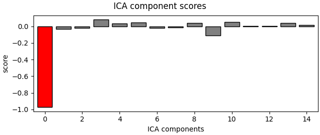
# find which ICs match the EOG pattern
eog_indices, eog_scores = ica.find_bads_eog(raw)
ica.exclude = eog_indices

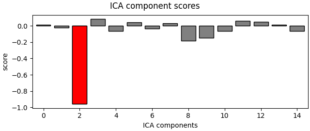
# barplot of ICA component "EOG match" scores
ica.plot_scores(eog_scores)

# plot diagnostics
ica.plot_properties(raw, picks=eog_indices)

# plot ICs applied to raw data, with EOG matches highlighted
ica.plot_sources(raw, show_scrollbars=False)

# plot ICs applied to the averaged EOG epochs, with EOG matches highlighted
ica.plot_sources(eog_evoked)

• 
• 
• 

Using EOG channel: EOG 061
... filtering ICA sources
Setting up band-pass filter from 1 - 10 Hz

FIR filter parameters
---------------------
Designing a two-pass forward and reverse, zero-phase, non-causal bandpass filter:
- Windowed frequency-domain design (firwin2) method
- Hann window
- Lower passband edge: 1.00
- Lower transition bandwidth: 0.50 Hz (-12 dB cutoff frequency: 0.75 Hz)
- Upper passband edge: 10.00 Hz
- Upper transition bandwidth: 0.50 Hz (-12 dB cutoff frequency: 10.25 Hz)
- Filter length: 1502 samples (10.003 s)

... filtering target
Setting up band-pass filter from 1 - 10 Hz

FIR filter parameters
---------------------
Designing a two-pass forward and reverse, zero-phase, non-causal bandpass filter:
- Windowed frequency-domain design (firwin2) method
- Hann window
- Lower passband edge: 1.00
- Lower transition bandwidth: 0.50 Hz (-12 dB cutoff frequency: 0.75 Hz)
- Upper passband edge: 10.00 Hz
- Upper transition bandwidth: 0.50 Hz (-12 dB cutoff frequency: 10.25 Hz)
- Filter length: 1502 samples (10.003 s)

    Using multitaper spectrum estimation with 7 DPSS windows
Not setting metadata
30 matching events found
No baseline correction applied
0 projection items activated
Creating RawArray with float64 data, n_channels=16, n_times=9010
    Range : 6450 ... 15459 =     42.956 ...   102.954 secs
Ready.

Note that above we used plot_sources() on both the original Raw instance and also on an Evoked instance of the extracted EOG artifacts. This can be another way to confirm that find_bads_eog() has identified the correct components.

Using a simulated channel to select ICA components

If you don’t have an EOG channel, find_bads_eog has a ch_name parameter that you can use as a proxy for EOG. You can use a single channel, or create a bipolar reference from frontal EEG sensors and use that as virtual EOG channel. This carries a risk however: you must hope that the frontal EEG channels only reflect EOG and not brain dynamics in the prefrontal cortex (or you must not care about those prefrontal signals).

For ECG, it is easier: find_bads_ecg can use cross-channel averaging of magnetometer or gradiometer channels to construct a virtual ECG channel, so if you have MEG channels it is usually not necessary to pass a specific channel name. find_bads_ecg also has two options for its method parameter: 'ctps' (cross-trial phase statistics [3]) and 'correlation' (Pearson correlation between data and ECG channel).

ica.exclude = []
# find which ICs match the ECG pattern
ecg_indices, ecg_scores = ica.find_bads_ecg(raw, method="correlation", threshold="auto")
ica.exclude = ecg_indices

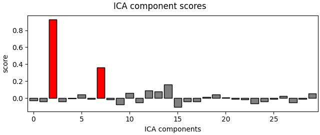
# barplot of ICA component "ECG match" scores
ica.plot_scores(ecg_scores)

# plot diagnostics
ica.plot_properties(raw, picks=ecg_indices)

# plot ICs applied to raw data, with ECG matches highlighted
ica.plot_sources(raw, show_scrollbars=False)

# plot ICs applied to the averaged ECG epochs, with ECG matches highlighted
ica.plot_sources(ecg_evoked)

• 
• 
• 

Reconstructing ECG signal from Magnetometers
... filtering ICA sources
Setting up band-pass filter from 8 - 16 Hz

FIR filter parameters
---------------------
Designing a two-pass forward and reverse, zero-phase, non-causal bandpass filter:
- Windowed frequency-domain design (firwin2) method
- Hann window
- Lower passband edge: 8.00
- Lower transition bandwidth: 0.50 Hz (-12 dB cutoff frequency: 7.75 Hz)
- Upper passband edge: 16.00 Hz
- Upper transition bandwidth: 0.50 Hz (-12 dB cutoff frequency: 16.25 Hz)
- Filter length: 1502 samples (10.003 s)

... filtering target
Setting up band-pass filter from 8 - 16 Hz

FIR filter parameters
---------------------
Designing a two-pass forward and reverse, zero-phase, non-causal bandpass filter:
- Windowed frequency-domain design (firwin2) method
- Hann window
- Lower passband edge: 8.00
- Lower transition bandwidth: 0.50 Hz (-12 dB cutoff frequency: 7.75 Hz)
- Upper passband edge: 16.00 Hz
- Upper transition bandwidth: 0.50 Hz (-12 dB cutoff frequency: 16.25 Hz)
- Filter length: 1502 samples (10.003 s)

    Using multitaper spectrum estimation with 7 DPSS windows
Not setting metadata
30 matching events found
No baseline correction applied
0 projection items activated
Creating RawArray with float64 data, n_channels=16, n_times=9010
    Range : 6450 ... 15459 =     42.956 ...   102.954 secs
Ready.

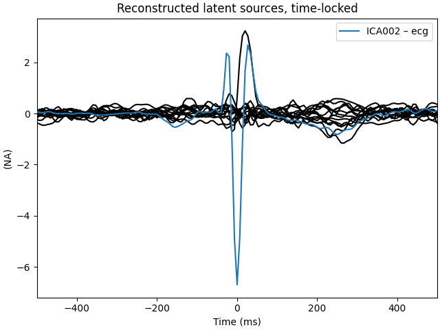
The last of these plots is especially useful: it shows us that the heartbeat artifact is coming through on two ICs, and we’ve only caught one of them. In fact, if we look closely at the output of plot_sources (online, you can right-click → “view image” to zoom in), it looks like ICA014 has a weak periodic component that is in-phase with ICA001. It might be worthwhile to re-run the ICA with more components to see if that second heartbeat artifact resolves out a little better:

# refit the ICA with 30 components this time
new_ica = ICA(n_components=30, max_iter="auto", random_state=97)
new_ica.fit(filt_raw)

# find which ICs match the ECG pattern
ecg_indices, ecg_scores = new_ica.find_bads_ecg(
    raw, method="correlation", threshold="auto"
)
new_ica.exclude = ecg_indices

# barplot of ICA component "ECG match" scores
new_ica.plot_scores(ecg_scores)

# plot diagnostics
new_ica.plot_properties(raw, picks=ecg_indices)

# plot ICs applied to raw data, with ECG matches highlighted
new_ica.plot_sources(raw, show_scrollbars=False)

# plot ICs applied to the averaged ECG epochs, with ECG matches highlighted
new_ica.plot_sources(ecg_evoked)

• 
• 
• 
• 

Fitting ICA to data using 161 channels (please be patient, this may take a while)
Selecting by number: 30 components
Fitting ICA took 0.5s.
Reconstructing ECG signal from Magnetometers
... filtering ICA sources
Setting up band-pass filter from 8 - 16 Hz

FIR filter parameters
---------------------
Designing a two-pass forward and reverse, zero-phase, non-causal bandpass filter:
- Windowed frequency-domain design (firwin2) method
- Hann window
- Lower passband edge: 8.00
- Lower transition bandwidth: 0.50 Hz (-12 dB cutoff frequency: 7.75 Hz)
- Upper passband edge: 16.00 Hz
- Upper transition bandwidth: 0.50 Hz (-12 dB cutoff frequency: 16.25 Hz)
- Filter length: 1502 samples (10.003 s)

[Parallel(n_jobs=1)]: Done  17 tasks      | elapsed:    0.0s
... filtering target
Setting up band-pass filter from 8 - 16 Hz

FIR filter parameters
---------------------
Designing a two-pass forward and reverse, zero-phase, non-causal bandpass filter:
- Windowed frequency-domain design (firwin2) method
- Hann window
- Lower passband edge: 8.00
- Lower transition bandwidth: 0.50 Hz (-12 dB cutoff frequency: 7.75 Hz)
- Upper passband edge: 16.00 Hz
- Upper transition bandwidth: 0.50 Hz (-12 dB cutoff frequency: 16.25 Hz)
- Filter length: 1502 samples (10.003 s)

    Using multitaper spectrum estimation with 7 DPSS windows
Not setting metadata
30 matching events found
No baseline correction applied
0 projection items activated
Not setting metadata
30 matching events found
No baseline correction applied
0 projection items activated
Creating RawArray with float64 data, n_channels=31, n_times=9010
    Range : 6450 ... 15459 =     42.956 ...   102.954 secs
Ready.

Much better! Now we’ve captured both ICs that are reflecting the heartbeat artifact (and as a result, we got two diagnostic plots: one for each IC that reflects the heartbeat). This demonstrates the value of checking the results of automated approaches like find_bads_ecg before accepting them.

For EEG, activation of muscles for postural control of the head and neck contaminate the signal as well. This is usually not detected by MEG. For an example showing how to remove these components, see Removing muscle ICA components.

# clean up memory before moving on
del raw, ica, new_ica

Selecting ICA components using template matching

When dealing with multiple subjects, it is also possible to manually select an IC for exclusion on one subject, and then use that component as a template for selecting which ICs to exclude from other subjects’ data, using mne.preprocessing.corrmap [4]. The idea behind corrmap is that the artifact patterns are similar enough across subjects that corresponding ICs can be identified by correlating the ICs from each ICA solution with a common template, and picking the ICs with the highest correlation strength. corrmap takes a list of ICA solutions, and a template parameter that specifies which ICA object and which component within it to use as a template.

Since our sample dataset only contains data from one subject, we’ll use a different dataset with multiple subjects: the EEGBCI dataset [5][6]. The dataset has 109 subjects, we’ll just download one run (a left/right hand movement task) from each of the first 4 subjects:

raws = list()
icas = list()

for subj in range(1, 5):
    # EEGBCI subjects are 1-indexed; run 3 is a left/right hand movement task
    fname = mne.datasets.eegbci.load_data(subj, runs=[3])[0]
    raw = mne.io.read_raw_edf(fname).load_data().resample(50)
    # remove trailing `.` from channel names so we can set montage
    mne.datasets.eegbci.standardize(raw)
    raw.set_montage("standard_1005")
    # high-pass filter
    raw_filt = raw.copy().load_data().filter(l_freq=1.0, h_freq=None)
    # fit ICA, using low max_iter for speed
    ica = ICA(n_components=30, max_iter=100, random_state=97)
    ica.fit(raw_filt, verbose="error")
    raws.append(raw)
    icas.append(ica)

Extracting EDF parameters from /home/circleci/mne_data/MNE-eegbci-data/files/eegmmidb/1.0.0/S001/S001R03.edf...
EDF file detected
Setting channel info structure...
Creating raw.info structure...
Reading 0 ... 19999  =      0.000 ...   124.994 secs...
Filtering raw data in 1 contiguous segment
Setting up high-pass filter at 1 Hz

FIR filter parameters
---------------------
Designing a one-pass, zero-phase, non-causal highpass filter:
- Windowed time-domain design (firwin) method
- Hamming window with 0.0194 passband ripple and 53 dB stopband attenuation
- Lower passband edge: 1.00
- Lower transition bandwidth: 1.00 Hz (-6 dB cutoff frequency: 0.50 Hz)
- Filter length: 165 samples (3.300 s)

[Parallel(n_jobs=1)]: Done  17 tasks      | elapsed:    0.0s
Extracting EDF parameters from /home/circleci/mne_data/MNE-eegbci-data/files/eegmmidb/1.0.0/S002/S002R03.edf...
EDF file detected
Setting channel info structure...
Creating raw.info structure...
Reading 0 ... 19679  =      0.000 ...   122.994 secs...
Filtering raw data in 1 contiguous segment
Setting up high-pass filter at 1 Hz

FIR filter parameters
---------------------
Designing a one-pass, zero-phase, non-causal highpass filter:
- Windowed time-domain design (firwin) method
- Hamming window with 0.0194 passband ripple and 53 dB stopband attenuation
- Lower passband edge: 1.00
- Lower transition bandwidth: 1.00 Hz (-6 dB cutoff frequency: 0.50 Hz)
- Filter length: 165 samples (3.300 s)

[Parallel(n_jobs=1)]: Done  17 tasks      | elapsed:    0.0s
Extracting EDF parameters from /home/circleci/mne_data/MNE-eegbci-data/files/eegmmidb/1.0.0/S003/S003R03.edf...
EDF file detected
Setting channel info structure...
Creating raw.info structure...
Reading 0 ... 19999  =      0.000 ...   124.994 secs...
Filtering raw data in 1 contiguous segment
Setting up high-pass filter at 1 Hz

FIR filter parameters
---------------------
Designing a one-pass, zero-phase, non-causal highpass filter:
- Windowed time-domain design (firwin) method
- Hamming window with 0.0194 passband ripple and 53 dB stopband attenuation
- Lower passband edge: 1.00
- Lower transition bandwidth: 1.00 Hz (-6 dB cutoff frequency: 0.50 Hz)
- Filter length: 165 samples (3.300 s)

[Parallel(n_jobs=1)]: Done  17 tasks      | elapsed:    0.0s
/home/circleci/python_env/lib/python3.12/site-packages/sklearn/decomposition/_fastica.py:128: ConvergenceWarning: FastICA did not converge. Consider increasing tolerance or the maximum number of iterations.
  warnings.warn(
Extracting EDF parameters from /home/circleci/mne_data/MNE-eegbci-data/files/eegmmidb/1.0.0/S004/S004R03.edf...
EDF file detected
Setting channel info structure...
Creating raw.info structure...
Reading 0 ... 19679  =      0.000 ...   122.994 secs...
Filtering raw data in 1 contiguous segment
Setting up high-pass filter at 1 Hz

FIR filter parameters
---------------------
Designing a one-pass, zero-phase, non-causal highpass filter:
- Windowed time-domain design (firwin) method
- Hamming window with 0.0194 passband ripple and 53 dB stopband attenuation
- Lower passband edge: 1.00
- Lower transition bandwidth: 1.00 Hz (-6 dB cutoff frequency: 0.50 Hz)
- Filter length: 165 samples (3.300 s)

[Parallel(n_jobs=1)]: Done  17 tasks      | elapsed:    0.0s
/home/circleci/python_env/lib/python3.12/site-packages/sklearn/decomposition/_fastica.py:128: ConvergenceWarning: FastICA did not converge. Consider increasing tolerance or the maximum number of iterations.
  warnings.warn(

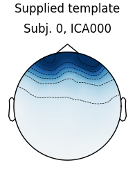
Now let’s run corrmap:

# use the first subject as template; use Fpz as proxy for EOG
raw = raws[0]
ica = icas[0]
eog_inds, eog_scores = ica.find_bads_eog(raw, ch_name="Fpz")
corrmap(icas, template=(0, eog_inds[0]))

• 
• 

Using EOG channel: Fpz
... filtering ICA sources
Setting up band-pass filter from 1 - 10 Hz

FIR filter parameters
---------------------
Designing a two-pass forward and reverse, zero-phase, non-causal bandpass filter:
- Windowed frequency-domain design (firwin2) method
- Hann window
- Lower passband edge: 1.00
- Lower transition bandwidth: 0.50 Hz (-12 dB cutoff frequency: 0.75 Hz)
- Upper passband edge: 10.00 Hz
- Upper transition bandwidth: 0.50 Hz (-12 dB cutoff frequency: 10.25 Hz)
- Filter length: 500 samples (10.000 s)

[Parallel(n_jobs=1)]: Done  17 tasks      | elapsed:    0.0s
... filtering target
Setting up band-pass filter from 1 - 10 Hz

FIR filter parameters
---------------------
Designing a two-pass forward and reverse, zero-phase, non-causal bandpass filter:
- Windowed frequency-domain design (firwin2) method
- Hann window
- Lower passband edge: 1.00
- Lower transition bandwidth: 0.50 Hz (-12 dB cutoff frequency: 0.75 Hz)
- Upper passband edge: 10.00 Hz
- Upper transition bandwidth: 0.50 Hz (-12 dB cutoff frequency: 10.25 Hz)
- Filter length: 500 samples (10.000 s)

Median correlation with constructed map: 0.978
Displaying selected ICs per subject.
At least 1 IC detected for each subject.

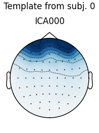
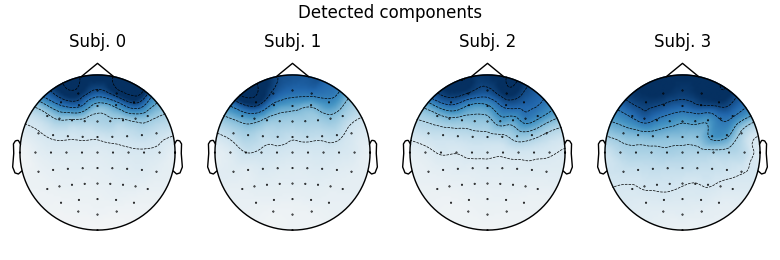
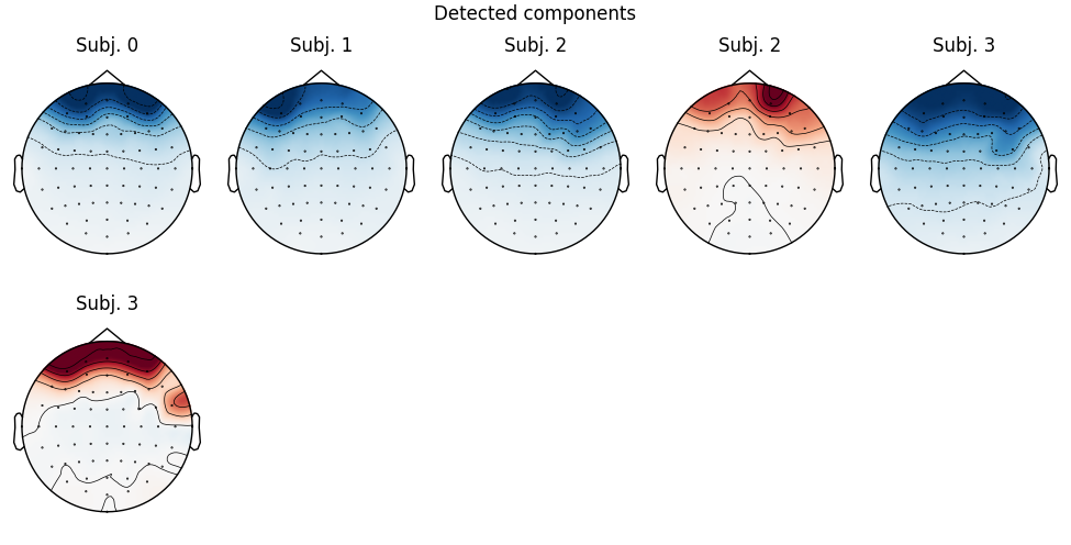
The first figure shows the template map, while the second figure shows all the maps that were considered a “match” for the template (including the template itself). There is one match for each subject, but it’s a good idea to also double-check the ICA sources for each subject:

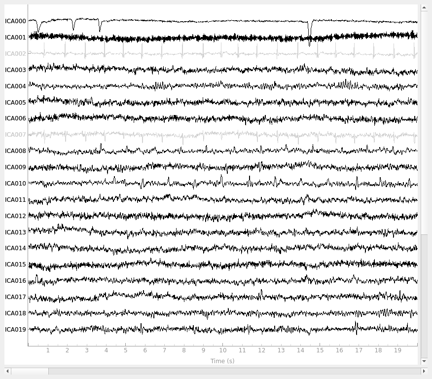
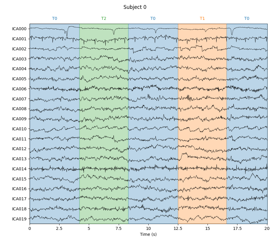
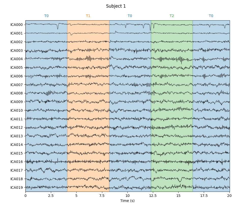
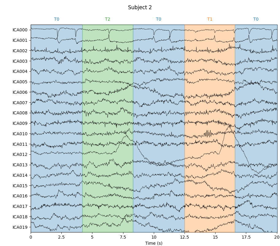
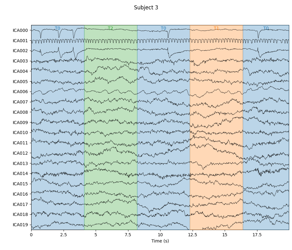
for index, (ica, raw) in enumerate(zip(icas, raws)):
    with mne.viz.use_browser_backend("matplotlib"):
        fig = ica.plot_sources(raw, show_scrollbars=False)
    fig.subplots_adjust(top=0.9)  # make space for title
    fig.suptitle(f"Subject {index}")

• 
• 
• 
• 

Using matplotlib as 2D backend.
Creating RawArray with float64 data, n_channels=30, n_times=6250
    Range : 0 ... 6249 =      0.000 ...   124.980 secs
Ready.
Using qt as 2D backend.
Using matplotlib as 2D backend.
Creating RawArray with float64 data, n_channels=30, n_times=6150
    Range : 0 ... 6149 =      0.000 ...   122.980 secs
Ready.
Using qt as 2D backend.
Using matplotlib as 2D backend.
Creating RawArray with float64 data, n_channels=30, n_times=6250
    Range : 0 ... 6249 =      0.000 ...   124.980 secs
Ready.
Using qt as 2D backend.
Using matplotlib as 2D backend.
Creating RawArray with float64 data, n_channels=30, n_times=6150
    Range : 0 ... 6149 =      0.000 ...   122.980 secs
Ready.
Using qt as 2D backend.

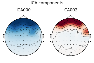
Notice that subjects 2 and 3 each seem to have two ICs that reflect ocular activity (components ICA000 and ICA002), but only one was caught by corrmap. Let’s try setting the threshold manually:

corrmap(icas, template=(0, eog_inds[0]), threshold=0.9)

• 
• 

Median correlation with constructed map: 0.958
Displaying selected ICs per subject.
At least 1 IC detected for each subject.

This time it found 2 ICs for each of subjects 2 and 3 (which is good). At this point we’ll re-run corrmap with parameters label='blink', plot=False to label the ICs from each subject that capture the blink artifacts (without plotting them again).

corrmap(icas, template=(0, eog_inds[0]), threshold=0.9, label="blink", plot=False)
print([ica.labels_ for ica in icas])

Median correlation with constructed map: 0.958
At least 1 IC detected for each subject.
[{'eog/0/Fpz': [np.int64(0)], 'eog': [np.int64(0)], 'blink': [np.int64(0)]}, {'blink': [np.int64(0)]}, {'blink': [np.int64(0), np.int64(1)]}, {'blink': [np.int64(0), np.int64(2)]}]

Notice that the first subject has 3 different labels for the IC at index 0: “eog/0/Fpz”, “eog”, and “blink”. The first two were added by find_bads_eog; the “blink” label was added by the last call to corrmap. Notice also that each subject has at least one IC index labelled “blink”, and subjects 2 and 3 each have two components (0 and 2) labelled “blink” (consistent with the plot of IC sources above). The labels_ attribute of ICA objects can also be manually edited to annotate the ICs with custom labels. They also come in handy when plotting:

icas[3].plot_components(picks=icas[3].labels_["blink"])
icas[3].exclude = icas[3].labels_["blink"]
icas[3].plot_sources(raws[3], show_scrollbars=False)

Creating RawArray with float64 data, n_channels=30, n_times=6150
    Range : 0 ... 6149 =      0.000 ...   122.980 secs
Ready.

As a final note, it is possible to extract ICs numerically using the get_components method of ICA objects. This will return a NumPy array that can be passed to corrmap instead of the tuple of (subject_index, component_index) we passed before, and will yield the same result:

template_eog_component = icas[0].get_components()[:, eog_inds[0]]
corrmap(icas, template=template_eog_component, threshold=0.9)
print(template_eog_component)

• 
• 

Median correlation with constructed map: 0.958
Displaying selected ICs per subject.
At least 1 IC detected for each subject.
[-0.33638605 -0.32708878 -0.32846765 -0.32807248 -0.35916344 -0.37615216
 -0.42464993 -0.21789139 -0.22387812 -0.22237922 -0.21342143 -0.2425263
 -0.26757238 -0.27806995 -0.15470616 -0.1693302  -0.17711037 -0.17373137
 -0.19651749 -0.21091786 -0.22459439 -1.68783519 -1.46717407 -1.64182737
 -1.34165002 -1.28991817 -0.76938995 -1.0057612  -1.54311043 -0.54567127
 -0.63806031 -0.57058636 -0.52637437 -0.51788659 -0.55774431 -0.56188149
 -0.69340923 -0.73333856 -0.2829121  -0.39253171 -0.16120286 -0.25431324
 -0.06352167 -0.1647002  -0.11930156 -0.1811579  -0.10112171 -0.12638332
 -0.13623739 -0.1301851  -0.14380943 -0.15329772 -0.1715539  -0.16560352
 -0.13293812 -0.08175318 -0.10173655 -0.10764581 -0.12707317 -0.09785876
 -0.07433338 -0.08470678 -0.07373196 -0.03379354]

An advantage of using this numerical representation of an IC to capture a particular artifact pattern is that it can be saved and used as a template for future template-matching tasks using corrmap without having to load or recompute the ICA solution that yielded the template originally. Put another way, when the template is a NumPy array, the ICA object containing the template does not need to be in the list of ICAs provided to corrmap.

Compute ICA components on Epochs

ICA is now fit to epoched MEG data instead of the raw data. We assume that the non-stationary EOG artifacts have already been removed. The sources matching the ECG are automatically found and displayed.

Note

This example is computationally intensive, so it might take a few minutes to complete.

After reading the data, preprocessing consists of:

• MEG channel selection

• 1-30 Hz band-pass filter

• epoching -0.2 to 0.5 seconds with respect to events

• rejection based on peak-to-peak amplitude

Note that we don’t baseline correct the epochs here – we’ll do this after cleaning with ICA is completed. Baseline correction before ICA is not recommended by the MNE-Python developers, as it doesn’t guarantee optimal results.

filt_raw.pick(picks=["meg", "stim"], exclude="bads").load_data()
filt_raw.filter(1, 30, fir_design="firwin")

# peak-to-peak amplitude rejection parameters
reject = dict(mag=4e-12)
# create longer and more epochs for more artifact exposure
events = mne.find_events(filt_raw, stim_channel="STI 014")
# don't baseline correct epochs
epochs = mne.Epochs(
    filt_raw, events, event_id=None, tmin=-0.2, tmax=0.5, reject=reject, baseline=None
)

Filtering raw data in 1 contiguous segment
Setting up band-pass filter from 1 - 30 Hz

FIR filter parameters
---------------------
Designing a one-pass, zero-phase, non-causal bandpass filter:
- Windowed time-domain design (firwin) method
- Hamming window with 0.0194 passband ripple and 53 dB stopband attenuation
- Lower passband edge: 1.00
- Lower transition bandwidth: 1.00 Hz (-6 dB cutoff frequency: 0.50 Hz)
- Upper passband edge: 30.00 Hz
- Upper transition bandwidth: 7.50 Hz (-6 dB cutoff frequency: 33.75 Hz)
- Filter length: 497 samples (3.310 s)

[Parallel(n_jobs=1)]: Done  17 tasks      | elapsed:    0.0s
[Parallel(n_jobs=1)]: Done  71 tasks      | elapsed:    0.0s
86 events found on stim channel STI 014
Event IDs: [ 1  2  3  4  5 32]
Not setting metadata
86 matching events found
No baseline correction applied
Created an SSP operator (subspace dimension = 3)
3 projection items activated

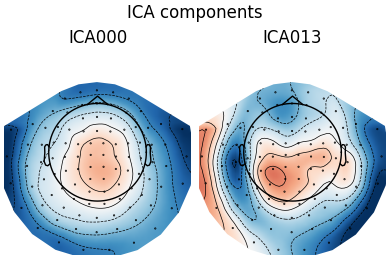
Fit ICA model using the FastICA algorithm, detect and plot components explaining ECG artifacts.

ica = ICA(n_components=15, method="fastica", max_iter="auto").fit(epochs)

ecg_epochs = create_ecg_epochs(filt_raw, tmin=-0.5, tmax=0.5)
ecg_inds, scores = ica.find_bads_ecg(ecg_epochs, threshold="auto")

ica.plot_components(ecg_inds)

Fitting ICA to data using 102 channels (please be patient, this may take a while)
Using data from preloaded Raw for 86 events and 106 original time points ...
0 bad epochs dropped
    Applying projection operator with 3 vectors (pre-whitener computation)
    Applying projection operator with 3 vectors (pre-whitener application)
Selecting by number: 15 components
Using data from preloaded Raw for 86 events and 106 original time points ...
    Applying projection operator with 3 vectors (pre-whitener application)
Fitting ICA took 0.3s.
Reconstructing ECG signal from Magnetometers
Setting up band-pass filter from 8 - 16 Hz

FIR filter parameters
---------------------
Designing a two-pass forward and reverse, zero-phase, non-causal bandpass filter:
- Windowed frequency-domain design (firwin2) method
- Hann window
- Lower passband edge: 8.00
- Lower transition bandwidth: 0.50 Hz (-12 dB cutoff frequency: 7.75 Hz)
- Upper passband edge: 16.00 Hz
- Upper transition bandwidth: 0.50 Hz (-12 dB cutoff frequency: 16.25 Hz)
- Filter length: 1502 samples (10.003 s)

Number of ECG events detected : 59 (average pulse 58.99492412402019 / min.)
Not setting metadata
59 matching events found
No baseline correction applied
Created an SSP operator (subspace dimension = 3)
Using data from preloaded Raw for 59 events and 151 original time points ...
0 bad epochs dropped
Reconstructing ECG signal from Magnetometers
Using threshold: 0.41 for CTPS ECG detection
    Applying projection operator with 3 vectors (pre-whitener application)

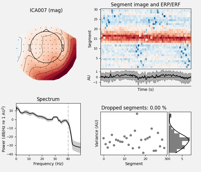
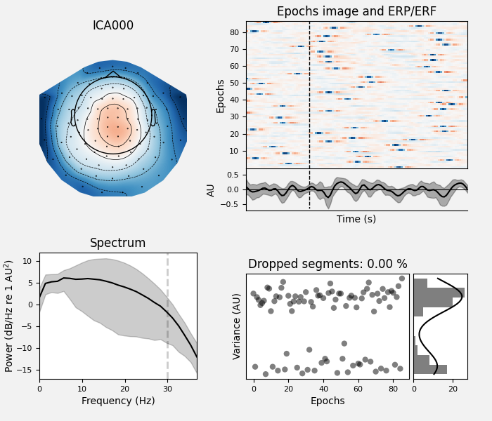
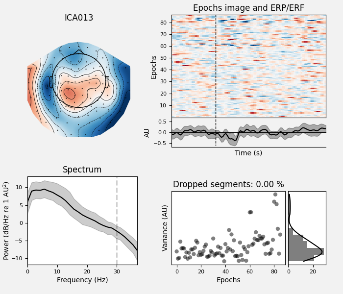
Plot the properties of the ECG components:

ica.plot_properties(epochs, picks=ecg_inds)

• 
• 

Using data from preloaded Raw for 86 events and 106 original time points ...
    Applying projection operator with 3 vectors (pre-whitener application)
    Using multitaper spectrum estimation with 7 DPSS windows
Not setting metadata
86 matching events found
No baseline correction applied
0 projection items activated
Not setting metadata
86 matching events found
No baseline correction applied
0 projection items activated

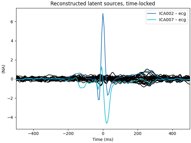
Plot the estimated sources of detected ECG related components:

ica.plot_sources(filt_raw, picks=ecg_inds)

    Applying projection operator with 3 vectors (pre-whitener application)
Creating RawArray with float64 data, n_channels=2, n_times=9010
    Range : 6450 ... 15459 =     42.956 ...   102.954 secs
Ready.

References

[1]

Pierre Ablin, Jean-Francois Cardoso, and Alexandre Gramfort. Faster Independent Component Analysis by preconditioning with hessian approximations. IEEE Transactions on Signal Processing, 66(15):4040–4049, 2018. doi:10.1109/TSP.2018.2844203.

[2]

Irene Winkler, Stefan Debener, Klaus-Robert Müller, and Michael Tangermann. On the influence of high-pass filtering on ICA-based artifact reduction in EEG-ERP. In Proceedings of EMBC-2015, 4101–4105. Milan, 2015. IEEE. doi:10.1109/EMBC.2015.7319296.

[3]

Jürgen Dammers, Michael Schiek, Frank Boers, Carmen Silex, Mikhail Zvyagintsev, Uwe Pietrzyk, and Klaus Mathiak. Integration of amplitude and phase statistics for complete artifact removal in independent components of neuromagnetic recordings. IEEE Transactions on Biomedical Engineering, 55(10):2353–2362, 2008. doi:10.1109/TBME.2008.926677.

[4]

Filipa Campos Viola, Jeremy Thorne, Barrie Edmonds, Till Schneider, Tom Eichele, and Stefan Debener. Semi-automatic identification of independent components representing EEG artifact. Clinical Neurophysiology, 120(5):868–877, 2009. doi:10.1016/j.clinph.2009.01.015.

[5]

Gerwin Schalk, Dennis J. McFarland, Thilo Hinterberger, Niels Birbaumer, and Jonathan R. Wolpaw. BCI2000: a general-purpose brain-computer interface (BCI) system. IEEE Transactions on Biomedical Engineering, 51(6):1034–1043, 2004. doi:10.1109/TBME.2004.827072.

[6]

Ary L. Goldberger, Luis A. N. Amaral, Leon Glass, Jeffrey M. Hausdorff, Plamen Ch. Ivanov, Roger G. Mark, Joseph E. Mietus, George B. Moody, Chung-Kang Peng, and H. Eugene Stanley. PhysioBank, PhysioToolkit, and PhysioNet: Components of a new research resource for complex physiologic signals. Circulation, 2000. doi:10.1161/01.CIR.101.23.e215.