Note
Go to the end to download the full example code.
Brainstorm Elekta phantom dataset tutorial#
This tutorial provides a step-by-step guide to importing and processing Elekta-Neuromag current phantom recordings.
A phantom recording is a measurement obtained using a device (phantom) that generates known magnetic signals, allowing validation and benchmarking of MEG system accuracy and analysis methods.
The aim of this tutorial is to demonstrate how phantom recordings can be used to evaluate source localisation methods by comparing estimated and true dipole positions.
For comparison, see [1] and the original Brainstorm tutorial.
# Authors: Eric Larson <larson.eric.d@gmail.com>
#          Carina Forster <carinaforster0611@gmail.com>
#
# License: BSD-3-Clause
# Copyright the MNE-Python contributors.
import matplotlib.pyplot as plt
import numpy as np
from scipy.signal import find_peaks

import mne
from mne import find_events, fit_dipole
from mne.datasets import fetch_phantom
from mne.datasets.brainstorm import bst_phantom_elekta
from mne.io import read_raw_fif
Load and prepare the data#
The data were collected with an Elekta Neuromag VectorView system at 1000 Hz, low-pass filtered at 330 Hz and contain recordings at three current amplitudes (20, 200, and 2000 nAm). Here we load the medium-amplitude condition.
# Load the data
data_path = bst_phantom_elekta.data_path(verbose=True)
raw_fname = data_path / "kojak_all_200nAm_pp_no_chpi_no_ms_raw.fif"
raw = read_raw_fif(raw_fname)
# Mark known bad channels
raw.info["bads"] = ["MEG1933", "MEG2421"]
# The first 32 events correspond to dipole activations
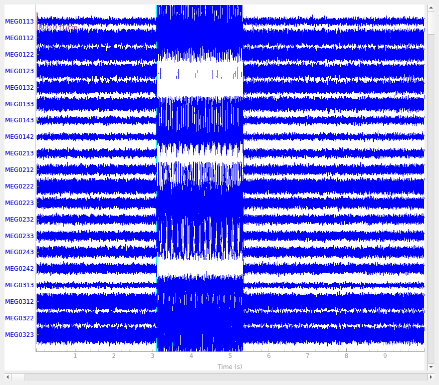
events = find_events(raw, "STI201")
Opening raw data file /home/circleci/mne_data/MNE-brainstorm-data/bst_phantom_elekta/kojak_all_200nAm_pp_no_chpi_no_ms_raw.fif...
    Read a total of 13 projection items:
        planar-0.0-115.0-PCA-01 (1 x 306)  idle
        planar-0.0-115.0-PCA-02 (1 x 306)  idle
        planar-0.0-115.0-PCA-03 (1 x 306)  idle
        planar-0.0-115.0-PCA-04 (1 x 306)  idle
        planar-0.0-115.0-PCA-05 (1 x 306)  idle
        axial-0.0-115.0-PCA-01 (1 x 306)  idle
        axial-0.0-115.0-PCA-02 (1 x 306)  idle
        axial-0.0-115.0-PCA-03 (1 x 306)  idle
        axial-0.0-115.0-PCA-04 (1 x 306)  idle
        axial-0.0-115.0-PCA-05 (1 x 306)  idle
        axial-0.0-115.0-PCA-06 (1 x 306)  idle
        axial-0.0-115.0-PCA-07 (1 x 306)  idle
        axial-0.0-115.0-PCA-08 (1 x 306)  idle
    Range : 47000 ... 437999 =     47.000 ...   437.999 secs
Ready.
Finding events on: STI201
645 events found on stim channel STI201
Event IDs: [   1    2    3    4    5    6    7    8    9   10   11   12   13   14
   15   16   17   18   19   20   21   22   23   24   25   26   27   28
   29   30   31   32  256  768 1792 3840 7936]
Epoch the data and plot evokeds#
We epoch and baseline correct the data around the dipole events.
# Epoch the data
bmax = -0.05
tmin, tmax = -0.1, 0.8
event_id = list(range(1, 33))
epochs = mne.Epochs(
    raw, events, event_id, tmin, tmax, baseline=(None, bmax), preload=False
)

# We drop the first and last event, it can contain dipole-switching artifacts
epochs_clean = epochs[1:-1]

# We select the first simulated dipole for visualisation purposes
epochs_firstdip = epochs_clean["1"]
Not setting metadata
640 matching events found
Setting baseline interval to [-0.1, -0.05] s
Applying baseline correction (mode: mean)
Created an SSP operator (subspace dimension = 13)
13 projection items activated
Let’s look at the evoked response for the first clean dipole.
We can see that the phantom was set to produce 20 Hz sinusoidal bursts of current and the burst envelope repeats at approximately 3 Hz.
epochs_firstdip.average().plot(time_unit="s")
Determine peak activation using Global Field Power (GFP)#
GFP is the standard deviation across sensors at each time point, providing a reference-independent measure of signal strength.
# Get the evoked signal of the first dipole
evoked_tmp = epochs_firstdip.average()

# Calculate GFP
gfp = np.std(evoked_tmp.data, axis=0)

# Restrict to first burst window
times = evoked_tmp.times
time_mask = (times > 0) & (times <= 0.05)

# Find the peak GFP indices
peaks, _ = find_peaks(gfp[time_mask])
peak_indices = np.where(time_mask)[0][peaks]

# Select the strongest peak
strongest_peak_idx = peak_indices[np.argmax(gfp[peak_indices])]
t_peak = times[strongest_peak_idx]
print(f"Strongest peak at {t_peak * 1000:.1f} ms")
Strongest peak at 37.0 ms
Here we select the peak amplitude timepoint and store the evoked data for each dipole.
evokeds = []
for ii in event_id:
    evoked = epochs_clean[str(ii)].average().crop(t_peak, t_peak)
    evoked = mne.EvokedArray(np.array(evoked.data), evoked.info, tmin=0.0)
    evokeds.append(evoked)
Next, we need to compute the noise covariance in the baseline window to capture the sensor noise structure (for details: Computing a covariance matrix).
cov = mne.compute_covariance(epochs_clean, tmax=bmax)
del epochs  # delete to save memory
Loading data for 19 events and 901 original time points ...
0 bad epochs dropped
Loading data for 20 events and 901 original time points ...
0 bad epochs dropped
Loading data for 20 events and 901 original time points ...
0 bad epochs dropped
Loading data for 20 events and 901 original time points ...
0 bad epochs dropped
Loading data for 20 events and 901 original time points ...
0 bad epochs dropped
Loading data for 20 events and 901 original time points ...
0 bad epochs dropped
Loading data for 20 events and 901 original time points ...
0 bad epochs dropped
Loading data for 20 events and 901 original time points ...
0 bad epochs dropped
Loading data for 20 events and 901 original time points ...
0 bad epochs dropped
Loading data for 20 events and 901 original time points ...
0 bad epochs dropped
Loading data for 20 events and 901 original time points ...
0 bad epochs dropped
Loading data for 20 events and 901 original time points ...
0 bad epochs dropped
Loading data for 20 events and 901 original time points ...
0 bad epochs dropped
Loading data for 20 events and 901 original time points ...
0 bad epochs dropped
Loading data for 20 events and 901 original time points ...
0 bad epochs dropped
Loading data for 20 events and 901 original time points ...
0 bad epochs dropped
Loading data for 20 events and 901 original time points ...
0 bad epochs dropped
Loading data for 20 events and 901 original time points ...
0 bad epochs dropped
Loading data for 20 events and 901 original time points ...
0 bad epochs dropped
Loading data for 20 events and 901 original time points ...
0 bad epochs dropped
Loading data for 20 events and 901 original time points ...
0 bad epochs dropped
Loading data for 20 events and 901 original time points ...
0 bad epochs dropped
Loading data for 20 events and 901 original time points ...
0 bad epochs dropped
Loading data for 20 events and 901 original time points ...
0 bad epochs dropped
Loading data for 20 events and 901 original time points ...
0 bad epochs dropped
Loading data for 20 events and 901 original time points ...
0 bad epochs dropped
Loading data for 20 events and 901 original time points ...
0 bad epochs dropped
Loading data for 20 events and 901 original time points ...
0 bad epochs dropped
Loading data for 20 events and 901 original time points ...
0 bad epochs dropped
Loading data for 20 events and 901 original time points ...
0 bad epochs dropped
Loading data for 20 events and 901 original time points ...
0 bad epochs dropped
Loading data for 19 events and 901 original time points ...
0 bad epochs dropped
    Created an SSP operator (subspace dimension = 13)
    Setting small MEG eigenvalues to zero (without PCA)
Reducing data rank from 304 -> 291
Estimating covariance using EMPIRICAL
Done.
Number of samples used : 32538
[done]
We use a sphere head geometry model because the Elekta phantom is designed to approximate a spherical conductor with known dipole locations.
subjects_dir = data_path
fetch_phantom("otaniemi", subjects_dir=subjects_dir)
sphere = mne.make_sphere_model(r0=(0.0, 0.0, 0.0), head_radius=0.08)
0 files missing from phantom_otaniemi.txt in /home/circleci/mne_data/MNE-brainstorm-data/bst_phantom_elekta

Equiv. model fitting -> RV = 0.00349271 %%
mu1 = 0.944622    lambda1 = 0.137266
mu2 = 0.667574    lambda2 = 0.683311
mu3 = -0.294757    lambda3 = -0.0102081
Set up EEG sphere model with scalp radius    80.0 mm
Dipole fitting#
Finally, we fit dipoles for each phantom and store them in a list.
BEM : <ConductorModel | Sphere (3 layers): r0=[0.0, 0.0, 0.0] R=80 mm>
MRI transform : identity
Sphere model : origin at ( 0.00 0.00 0.00) mm, rad = 0.1 mm
Guess grid : 20.0 mm
Guess mindist : 5.0 mm
Guess exclude : 20.0 mm
Using normal MEG coil definitions.
Noise covariance : <Covariance | kind : full, shape : (304, 304), range : [-1.8e-21, +2.2e-21], n_samples : 32537>
Coordinate transformation: MRI (surface RAS) -> head
1.000000 0.000000 0.000000 0.00 mm
0.000000 1.000000 0.000000 0.00 mm
0.000000 0.000000 1.000000 0.00 mm
0.000000 0.000000 0.000000 1.00
Coordinate transformation: MEG device -> head
0.976295 -0.211976 0.043756 0.29 mm
0.206488 0.972764 0.105326 0.57 mm
-0.064891 -0.093794 0.993475 5.41 mm
0.000000 0.000000 0.000000 1.00
2 bad channels total
Read 304 MEG channels from info
105 coil definitions read
Coordinate transformation: MEG device -> head
0.976295 -0.211976 0.043756 0.29 mm
0.206488 0.972764 0.105326 0.57 mm
-0.064891 -0.093794 0.993475 5.41 mm
0.000000 0.000000 0.000000 1.00
MEG coil definitions created in head coordinates.
Decomposing the sensor noise covariance matrix...
Created an SSP operator (subspace dimension = 13)
Computing rank from covariance with rank=None
Using tolerance 5.7e-11 (2.2e-16 eps * 304 dim * 8.4e+02 max singular value)
Estimated rank (mag + grad): 291
MEG: rank 291 computed from 304 data channels with 13 projectors
Setting small MEG eigenvalues to zero (without PCA)
Created the whitener using a noise covariance matrix with rank 291 (13 small eigenvalues omitted)
---- Computing the forward solution for the guesses...
Making a spherical guess space with radius 72.0 mm...
Filtering (grid = 20 mm)...
Surface CM = ( 0.0 0.0 0.0) mm
Surface fits inside a sphere with radius 72.0 mm
Surface extent:
x = -72.0 ... 72.0 mm
y = -72.0 ... 72.0 mm
z = -72.0 ... 72.0 mm
Grid extent:
x = -80.0 ... 80.0 mm
y = -80.0 ... 80.0 mm
z = -80.0 ... 80.0 mm
729 sources before omitting any.
178 sources after omitting infeasible sources not within 20.0 - 72.0 mm.
Source spaces are in MRI coordinates.
Checking that the sources are inside the surface and at least 5.0 mm away (will take a few...)
8 source space point omitted because of the 5.0-mm distance limit.
170 sources remaining after excluding the sources outside the surface and less than 5.0 mm inside.
Go through all guess source locations...
[done 170 sources]
---- Fitted : 0.0 ms
Projections have already been applied. Setting proj attribute to True.
1 time points fitted
Evaluate goodness of fit#
The dipole object stores the goodness of fit (GOF) for each dipole. Some dipoles have a low GOF (< 60 %).
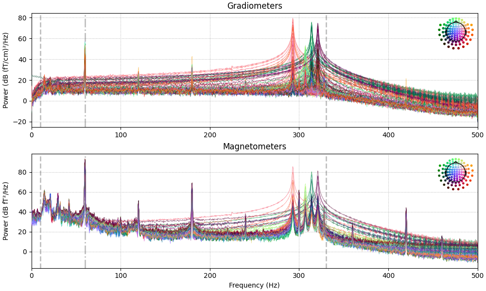
Dipoles with low goodness of fit#
Why do some dipoles have a low GOF? Here we plot the dipole locations of the dipoles with low GOF.
We can see that dipoles with low GOF are deep in the brain which might explain the low GOF.
# Get indices of low GOF dipoles
low_idx = [i for i, g in enumerate(gof) if g < 60]
low_event_ids = [event_id[i] for i in low_idx]

print("Low GOF dipoles:", low_event_ids)

# Let's plot the locations of the dipoles with low GOF.
low_dips = [dip_all[i] for i in low_idx]

subject = "phantom_otaniemi"
trans = mne.transforms.Transform("head", "mri", np.eye(4))

# Plot the position and the orientation of the dipoles with low GOF
fig = mne.viz.plot_alignment(
    evoked.info,
    trans,
    subject,
    bem=sphere,
    surfaces={"head-dense": 0.2},
    coord_frame="head",
    meg="helmet",
    show_axes=True,
    subjects_dir=subjects_dir,
)

fig = mne.viz.plot_dipole_locations(
    dipoles=low_dips, mode="arrow", subject=subject, color=(1.0, 0.2, 0.2), fig=fig
)

Low GOF dipoles: [4, 8, 28, 32]
Using lh.seghead for head surface.
Getting helmet for system 306m
Compare estimated and true dipoles#
The dipole fits closely match the true phantom data, achieving sub-centimeter accuracy (mean position error 2.4mm).
# We get the true dipole positions from the phantoms
actual_pos, actual_ori = mne.dipole.get_phantom_dipoles()
actual_amp = 100.0  # nAm

# Here we store the estimated dipoles
dip_pos = [dip.pos[0] for dip in dip_all]
dip_ori = [dip.ori[0] for dip in dip_all]
dip_amplitude = [dip.amplitude[0] for dip in dip_all]

fig, (ax1, ax2, ax3) = plt.subplots(
    nrows=3, ncols=1, figsize=(6, 7), layout="constrained"
)

# Here we calculate the euclidean distance between estimated and true positions.
# We multiply by 1000 to convert from meter to millimeter.
diffs = 1000 * np.sqrt(np.sum((dip_pos - actual_pos) ** 2, axis=-1))
print(f"mean(position error) = {np.mean(diffs):0.1f} mm")
ax1.bar(event_id, diffs)
ax1.set_xlabel("Dipole index")
ax1.set_ylabel("Loc. error (mm)")

# Next we calculate the angle between estimated and true orientation.
# We convert radians to degrees.
angles = np.rad2deg(np.arccos(np.abs(np.sum(dip_ori * actual_ori, axis=1))))
print(f"mean(angle error) = {np.mean(angles):0.1f}°")
ax2.bar(event_id, angles)
ax2.set_xlabel("Dipole index")
ax2.set_ylabel("Angle error (°)")

# Here we compare amplitudes by subtracting estimated from true amplitude.
amps = actual_amp - np.array(dip_amplitude) / 1e-9
print(f"mean(abs amplitude error) = {np.mean(np.abs(amps)):0.1f} nAm")
ax3.bar(event_id, amps)
ax3.set_xlabel("Dipole index")
ax3.set_ylabel("Amplitude error (nAm)")
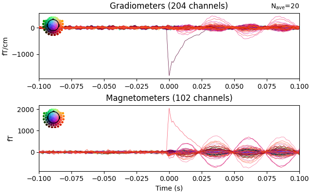
mean(position error) = 2.4 mm
mean(angle error) = 2.6°
mean(abs amplitude error) = 16.9 nAm
Visualise estimated and true dipole locations#
We can see that the dipoles overlap, have approximately the same magnitude and point in the same direction.
actual_amp = np.ones(len(dip))  # fake amp, needed to create Dipole instance
actual_gof = np.ones(len(dip))  # fake goodness-of-fit (GOF)
# setup dipole objects for true and estimated dipoles
dip_true = mne.Dipole(dip.times, actual_pos, actual_amp, actual_ori, actual_gof)
dip_estimated = mne.Dipole(dip.times, dip_pos, dip_amplitude, dip_ori, actual_gof)

fig = mne.viz.plot_alignment(
    evoked.info,
    trans,
    subject,
    bem=sphere,
    surfaces={"head-dense": 0.2},
    coord_frame="head",
    meg="helmet",
    show_axes=True,
    subjects_dir=subjects_dir,
)

# Plot the position and the orientation of the true dipole in black
fig = mne.viz.plot_dipole_locations(
    dipoles=dip_true, mode="arrow", subject=subject, color=(0.0, 0.0, 0.0), fig=fig
)

# Plot the position and the orientation of the estimated dipole in green
fig = mne.viz.plot_dipole_locations(
    dipoles=dip_estimated, mode="arrow", subject=subject, color=(0.2, 1.0, 0.5), fig=fig
)
mne.viz.set_3d_view(figure=fig, azimuth=70, elevation=80, distance=0.5)
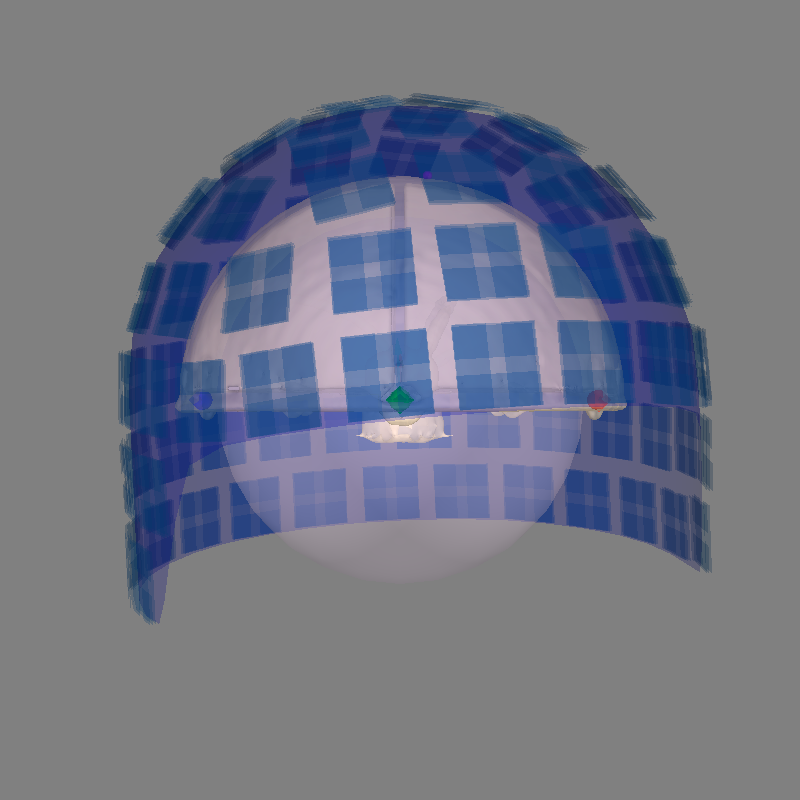
Using lh.seghead for head surface.
Getting helmet for system 306m
References#
Total running time of the script: (1 minutes 7.688 seconds)