Note
Go to the end to download the full example code.
Permutation t-test on source data with spatio-temporal clustering#
This example tests if the evoked response is significantly different between two conditions across subjects. Here just for demonstration purposes we simulate data from multiple subjects using one subject’s data. The multiple comparisons problem is addressed with a cluster-level permutation test across space and time.
# Authors: Alexandre Gramfort <alexandre.gramfort@inria.fr>
#          Eric Larson <larson.eric.d@gmail.com>
#          Stefan Appelhoff <stefan.appelhoff@mailbox.org>
#
# License: BSD-3-Clause
# Copyright the MNE-Python contributors.
import numpy as np
from numpy.random import randn
from scipy import stats as stats

import mne
from mne.datasets import sample
from mne.epochs import equalize_epoch_counts
from mne.minimum_norm import apply_inverse, read_inverse_operator
from mne.stats import spatio_temporal_cluster_1samp_test, summarize_clusters_stc
Set parameters#
data_path = sample.data_path()
meg_path = data_path / "MEG" / "sample"
raw_fname = meg_path / "sample_audvis_filt-0-40_raw.fif"
event_fname = meg_path / "sample_audvis_filt-0-40_raw-eve.fif"
subjects_dir = data_path / "subjects"
src_fname = subjects_dir / "fsaverage" / "bem" / "fsaverage-ico-5-src.fif"

tmin = -0.2
tmax = 0.3  # Use a lower tmax to reduce multiple comparisons

# Setup for reading the raw data
raw = mne.io.read_raw_fif(raw_fname)
events = mne.read_events(event_fname)
Opening raw data file /home/circleci/mne_data/MNE-sample-data/MEG/sample/sample_audvis_filt-0-40_raw.fif...
    Read a total of 4 projection items:
        PCA-v1 (1 x 10²)  idle
        PCA-v2 (1 x 10²)  idle
        PCA-v3 (1 x 10²)  idle
        Average EEG reference (1 x 60)  idle
    Range : 6450 ... 48149 =     42.956 ...   320.665 secs
Ready.
Read epochs for all channels, removing a bad one#
raw.info["bads"] += ["MEG 2443"]
picks = mne.pick_types(raw.info, meg=True, eog=True, exclude="bads")
event_id = 1  # L auditory
reject = dict(grad=1000e-13, mag=4000e-15, eog=150e-6)
epochs1 = mne.Epochs(
    raw,
    events,
    event_id,
    tmin,
    tmax,
    picks=picks,
    baseline=(None, 0),
    reject=reject,
    preload=True,
)

event_id = 3  # L visual
epochs2 = mne.Epochs(
    raw,
    events,
    event_id,
    tmin,
    tmax,
    picks=picks,
    baseline=(None, 0),
    reject=reject,
    preload=True,
)

# Equalize trial counts to eliminate bias (which would otherwise be
# introduced by the abs() performed below)
equalize_epoch_counts([epochs1, epochs2])
Not setting metadata
72 matching events found
Setting baseline interval to [-0.19979521315838786, 0.0] s
Applying baseline correction (mode: mean)
Created an SSP operator (subspace dimension = 3)
3 projection items activated
Loading data for 72 events and 76 original time points ...
    Rejecting  epoch based on EOG : ['EOG 061']
    Rejecting  epoch based on EOG : ['EOG 061']
    Rejecting  epoch based on EOG : ['EOG 061']
    Rejecting  epoch based on EOG : ['EOG 061']
    Rejecting  epoch based on MAG : ['MEG 1711']
    Rejecting  epoch based on EOG : ['EOG 061']
    Rejecting  epoch based on EOG : ['EOG 061']
    Rejecting  epoch based on EOG : ['EOG 061']
    Rejecting  epoch based on EOG : ['EOG 061']
9 bad epochs dropped
Not setting metadata
73 matching events found
Setting baseline interval to [-0.19979521315838786, 0.0] s
Applying baseline correction (mode: mean)
Created an SSP operator (subspace dimension = 3)
3 projection items activated
Loading data for 73 events and 76 original time points ...
    Rejecting  epoch based on EOG : ['EOG 061']
    Rejecting  epoch based on EOG : ['EOG 061']
    Rejecting  epoch based on EOG : ['EOG 061']
    Rejecting  epoch based on EOG : ['EOG 061']
    Rejecting  epoch based on GRAD : ['MEG 1333', 'MEG 1342']
    Rejecting  epoch based on EOG : ['EOG 061']
6 bad epochs dropped
Dropped 0 epochs:
Dropped 4 epochs: 10, 25, 26, 40
Transform to source space#
fname_inv = meg_path / "sample_audvis-meg-oct-6-meg-inv.fif"
snr = 3.0
lambda2 = 1.0 / snr**2
method = "dSPM"  # use dSPM method (could also be MNE, sLORETA, or eLORETA)
inverse_operator = read_inverse_operator(fname_inv)
sample_vertices = [s["vertno"] for s in inverse_operator["src"]]

# Let's average and compute inverse, resampling to speed things up
evoked1 = epochs1.average()
evoked1.resample(50, npad="auto")
condition1 = apply_inverse(evoked1, inverse_operator, lambda2, method)
evoked2 = epochs2.average()
evoked2.resample(50, npad="auto")
condition2 = apply_inverse(evoked2, inverse_operator, lambda2, method)

# Let's only deal with t > 0, cropping to reduce multiple comparisons
condition1.crop(0, None)
condition2.crop(0, None)
tmin = condition1.tmin
tstep = condition1.tstep * 1000  # convert to milliseconds
Reading inverse operator decomposition from /home/circleci/mne_data/MNE-sample-data/MEG/sample/sample_audvis-meg-oct-6-meg-inv.fif...
    Reading inverse operator info...
    [done]
    Reading inverse operator decomposition...
    [done]
    305 x 305 full covariance (kind = 1) found.
    Read a total of 4 projection items:
        PCA-v1 (1 x 10²) active
        PCA-v2 (1 x 10²) active
        PCA-v3 (1 x 10²) active
        Average EEG reference (1 x 60) active
    Noise covariance matrix read.
    22494 x 22494 diagonal covariance (kind = 2) found.
    Source covariance matrix read.
    22494 x 22494 diagonal covariance (kind = 6) found.
    Orientation priors read.
    22494 x 22494 diagonal covariance (kind = 5) found.
    Depth priors read.
    Did not find the desired covariance matrix (kind = 3)
    Reading a source space...
    Computing patch statistics...
    Patch information added...
    Distance information added...
    [done]
    Reading a source space...
    Computing patch statistics...
    Patch information added...
    Distance information added...
    [done]
    2 source spaces read
    Read a total of 4 projection items:
        PCA-v1 (1 x 10²) active
        PCA-v2 (1 x 10²) active
        PCA-v3 (1 x 10²) active
        Average EEG reference (1 x 60) active
    Source spaces transformed to the inverse solution coordinate frame
Preparing the inverse operator for use...
    Scaled noise and source covariance from nave = 1 to nave = 63
    Created the regularized inverter
    Created an SSP operator (subspace dimension = 3)
    Created the whitener using a noise covariance matrix with rank 302 (3 small eigenvalues omitted)
    Computing noise-normalization factors (dSPM)...
[done]
Applying inverse operator to "1"...
    Picked 305 channels from the data
    Computing inverse...
    Eigenleads need to be weighted ...
    Computing residual...
    Explained  69.4% variance
    Combining the current components...
    dSPM...
[done]
Preparing the inverse operator for use...
    Scaled noise and source covariance from nave = 1 to nave = 63
    Created the regularized inverter
    Created an SSP operator (subspace dimension = 3)
    Created the whitener using a noise covariance matrix with rank 302 (3 small eigenvalues omitted)
    Computing noise-normalization factors (dSPM)...
[done]
Applying inverse operator to "3"...
    Picked 305 channels from the data
    Computing inverse...
    Eigenleads need to be weighted ...
    Computing residual...
    Explained  70.7% variance
    Combining the current components...
    dSPM...
[done]
Transform to common cortical space#
Normally you would read in estimates across several subjects and morph them to the same cortical space (e.g., fsaverage). For example purposes, we will simulate this by just having each “subject” have the same response (just noisy in source space) here.
Note
Note that for 6 subjects with a two-sided statistical test, the minimum
significance under a permutation test is only
p = 1/(2 ** 6) = 0.015, which is large.
n_vertices_sample, n_times = condition1.data.shape
n_subjects = 6
print(f"Simulating data for {n_subjects} subjects.")

# Let's make sure our results replicate, so set the seed.
np.random.seed(0)
X = randn(n_vertices_sample, n_times, n_subjects, 2) * 10
X[:, :, :, 0] += condition1.data[:, :, np.newaxis]
X[:, :, :, 1] += condition2.data[:, :, np.newaxis]
Simulating data for 6 subjects.
It’s a good idea to spatially smooth the data, and for visualization purposes, let’s morph these to fsaverage, which is a grade 5 source space with vertices 0:10242 for each hemisphere. Usually you’d have to morph each subject’s data separately (and you might want to use morph_data instead), but here since all estimates are on ‘sample’ we can use one morph matrix for all the heavy lifting.
# Read the source space we are morphing to
src = mne.read_source_spaces(src_fname)
fsave_vertices = [s["vertno"] for s in src]
morph_mat = mne.compute_source_morph(
    src=inverse_operator["src"],
    subject_to="fsaverage",
    spacing=fsave_vertices,
    subjects_dir=subjects_dir,
).morph_mat

n_vertices_fsave = morph_mat.shape[0]

# We have to change the shape for the dot() to work properly
X = X.reshape(n_vertices_sample, n_times * n_subjects * 2)
print("Morphing data.")
X = morph_mat.dot(X)  # morph_mat is a sparse matrix
X = X.reshape(n_vertices_fsave, n_times, n_subjects, 2)
    Reading a source space...
    [done]
    Reading a source space...
    [done]
    2 source spaces read
surface source space present ...
Computing morph matrix...
    Left-hemisphere map read.
    Right-hemisphere map read.
    17 smooth iterations done.
    14 smooth iterations done.
[done]
[done]
Morphing data.
Finally, we want to compare the overall activity levels in each condition, the diff is taken along the last axis (condition). The negative sign makes it so condition1 > condition2 shows up as “red blobs” (instead of blue).
Find adjacency matrix#
For cluster-based permutation testing, we must define adjacency relations that govern which points can become members of the same cluster. While these relations are rather obvious for dimensions such as time or frequency they require a bit more work for spatial dimension such as channels or source vertices.
Here, to use an algorithm optimized for spatio-temporal clustering, we
just pass the spatial adjacency matrix (instead of spatio-temporal).
But note that clustering still takes place along the
temporal dimension and can be
controlled via the max_step parameter in
mne.stats.spatio_temporal_cluster_1samp_test().
If we wanted to specify an adjacency matrix for both space and time
explicitly we would have to use mne.stats.combine_adjacency(),
however for the present case, this is not needed.
print("Computing adjacency.")
adjacency = mne.spatial_src_adjacency(src)
Computing adjacency.
-- number of adjacent vertices : 20484
Compute statistic#
# Note that X needs to be a multi-dimensional array of shape
# observations (subjects) × time × space, so we permute dimensions
X = np.transpose(X, [2, 1, 0])

# Here we set a cluster forming threshold based on a p-value for
# the cluster based permutation test.
# We use a two-tailed threshold, the "1 - p_threshold" is needed
# because for two-tailed tests we must specify a positive threshold.
p_threshold = 0.001
df = n_subjects - 1  # degrees of freedom for the test
t_threshold = stats.distributions.t.ppf(1 - p_threshold / 2, df=df)

# Now let's actually do the clustering. This can take a long time...
print("Clustering.")
T_obs, clusters, cluster_p_values, H0 = clu = spatio_temporal_cluster_1samp_test(
    X,
    adjacency=adjacency,
    n_jobs=None,
    threshold=t_threshold,
    buffer_size=None,
    verbose=True,
)
Clustering.
stat_fun(H1): min=-31.563536574840377 max=62.79154693338157
Running initial clustering …
Found 368 clusters

  0%|          | Permuting (exact test) : 0/31 [00:00<?,       ?it/s]
  3%|▎         | Permuting (exact test) : 1/31 [00:00<00:01,   29.49it/s]
 10%|▉         | Permuting (exact test) : 3/31 [00:00<00:00,   44.73it/s]
 16%|█▌        | Permuting (exact test) : 5/31 [00:00<00:00,   49.83it/s]
 23%|██▎       | Permuting (exact test) : 7/31 [00:00<00:00,   52.39it/s]
 26%|██▌       | Permuting (exact test) : 8/31 [00:00<00:00,   47.37it/s]
 32%|███▏      | Permuting (exact test) : 10/31 [00:00<00:00,   49.62it/s]
 39%|███▊      | Permuting (exact test) : 12/31 [00:00<00:00,   51.20it/s]
 42%|████▏     | Permuting (exact test) : 13/31 [00:00<00:00,   48.00it/s]
 48%|████▊     | Permuting (exact test) : 15/31 [00:00<00:00,   49.53it/s]
 52%|█████▏    | Permuting (exact test) : 16/31 [00:00<00:00,   47.05it/s]
 55%|█████▍    | Permuting (exact test) : 17/31 [00:00<00:00,   45.03it/s]
 58%|█████▊    | Permuting (exact test) : 18/31 [00:00<00:00,   43.36it/s]
 61%|██████▏   | Permuting (exact test) : 19/31 [00:00<00:00,   41.95it/s]
 65%|██████▍   | Permuting (exact test) : 20/31 [00:00<00:00,   40.76it/s]
 68%|██████▊   | Permuting (exact test) : 21/31 [00:00<00:00,   39.73it/s]
 74%|███████▍  | Permuting (exact test) : 23/31 [00:00<00:00,   41.48it/s]
 77%|███████▋  | Permuting (exact test) : 24/31 [00:00<00:00,   40.47it/s]
 81%|████████  | Permuting (exact test) : 25/31 [00:00<00:00,   39.58it/s]
 84%|████████▍ | Permuting (exact test) : 26/31 [00:00<00:00,   38.78it/s]
 87%|████████▋ | Permuting (exact test) : 27/31 [00:00<00:00,   38.06it/s]
 90%|█████████ | Permuting (exact test) : 28/31 [00:00<00:00,   37.43it/s]
 94%|█████████▎| Permuting (exact test) : 29/31 [00:00<00:00,   36.86it/s]
 97%|█████████▋| Permuting (exact test) : 30/31 [00:00<00:00,   36.34it/s]
100%|██████████| Permuting (exact test) : 31/31 [00:00<00:00,   39.59it/s]
Selecting “significant” clusters#
After performing the cluster-based permutationt test, you may wish to select the observed clusters that can be considered statistically significant under the permutation distribution. This can easily be done using the code snippet below.
However, it is crucial to be aware that a statistically significant observed cluster does not directly translate into statistical significance of the channels, time points, frequency bins, etc. that form the cluster!
For more information, see the FieldTrip tutorial.
# Select the clusters that are statistically significant at p < 0.05
good_clusters_idx = np.where(cluster_p_values < 0.05)[0]
good_clusters = [clusters[idx] for idx in good_clusters_idx]
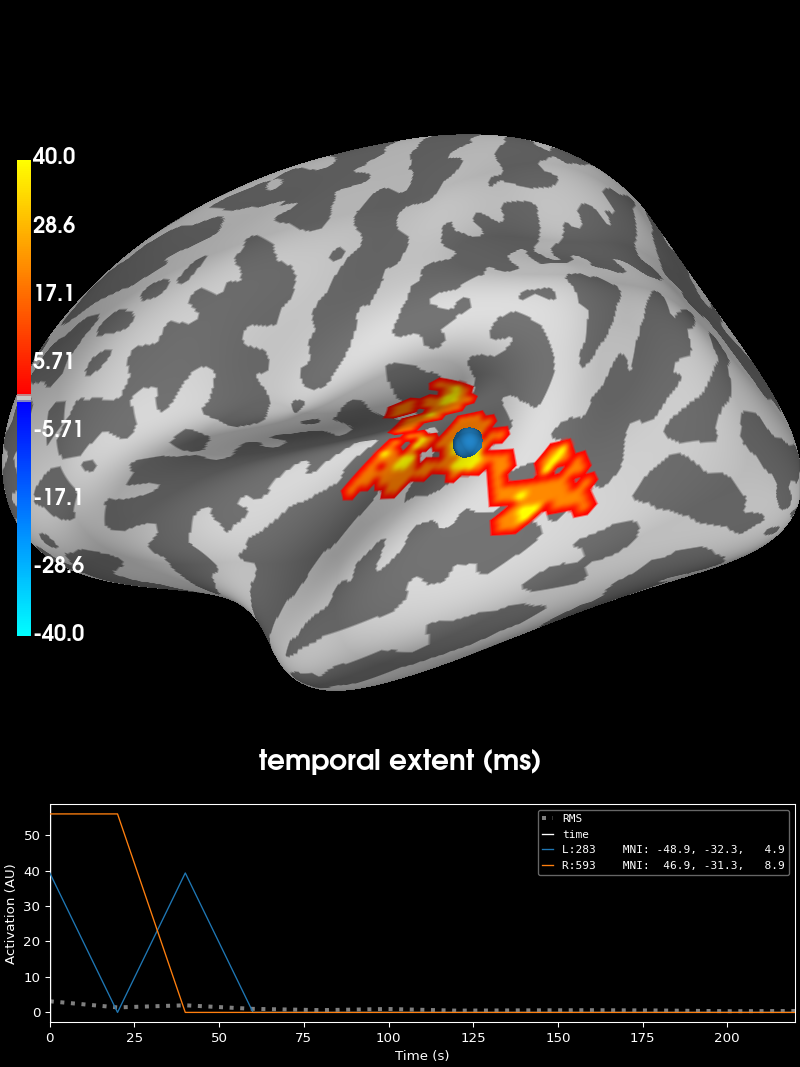
Visualize the clusters#
print("Visualizing clusters.")

# Now let's build a convenient representation of our results, where consecutive
# cluster spatial maps are stacked in the time dimension of a SourceEstimate
# object. This way by moving through the time dimension we will be able to see
# subsequent cluster maps.
stc_all_cluster_vis = summarize_clusters_stc(
    clu, tstep=tstep, vertices=fsave_vertices, subject="fsaverage"
)

# Let's actually plot the first "time point" in the SourceEstimate, which
# shows all the clusters, weighted by duration.

# blue blobs are for condition A < condition B, red for A > B
brain = stc_all_cluster_vis.plot(
    hemi="both",
    views="lateral",
    subjects_dir=subjects_dir,
    time_label="temporal extent (ms)",
    size=(800, 800),
    smoothing_steps=5,
    clim=dict(kind="value", pos_lims=[0, 1, 40]),
)

# We could save this via the following:
# brain.save_image('clusters.png')
Visualizing clusters.
Total running time of the script: (0 minutes 10.691 seconds)