Note

Go to the end to download the full example code.

Working with sEEG data#

MNE-Python supports working with more than just MEG and EEG data. Here we show some of the functions that can be used to facilitate working with stereoelectroencephalography (sEEG) data.

This example shows how to use:

sEEG data
channel locations in MNI space
projection into a volume

Note that our sample sEEG electrodes are already assumed to be in MNI space. If you want to map positions from your subject MRI space to MNI fsaverage space, you must apply the FreeSurfer’s talairach.xfm transform for your dataset. You can take a look at How MNE uses FreeSurfer’s outputs for more information.

For an example that involves ECoG data, channel locations in a subject-specific MRI, or projection into a surface, see Working with ECoG data. In the ECoG example, we show how to visualize surface grid channels on the brain.

Please note that this tutorial requires 3D plotting dependencies, see Install via pip or conda.

# Authors: Eric Larson <larson.eric.d@gmail.com>
#          Adam Li <adam2392@gmail.com>
#          Alex Rockhill <aprockhill@mailbox.org>
#
# License: BSD-3-Clause
# Copyright the MNE-Python contributors.

import numpy as np

import mne
from mne.datasets import fetch_fsaverage

# paths to mne datasets - sample sEEG and FreeSurfer's fsaverage subject
# which is in MNI space
misc_path = mne.datasets.misc.data_path()
sample_path = mne.datasets.sample.data_path()
subjects_dir = sample_path / "subjects"

# use mne-python's fsaverage data
fetch_fsaverage(subjects_dir=subjects_dir, verbose=True)  # downloads if needed

0 files missing from root.txt in /home/circleci/mne_data/MNE-sample-data/subjects
0 files missing from bem.txt in /home/circleci/mne_data/MNE-sample-data/subjects/fsaverage

Let’s load some sEEG data with channel locations and make epochs.

raw = mne.io.read_raw(misc_path / "seeg" / "sample_seeg_ieeg.fif")

epochs = mne.Epochs(raw, detrend=1, baseline=None)
epochs = epochs["Response"][0]  # just process one epoch of data for speed

Opening raw data file /home/circleci/mne_data/MNE-misc-data/seeg/sample_seeg_ieeg.fif...
    Range : 1310640 ... 1370605 =   1311.411 ...  1371.411 secs
Ready.
Used Annotations descriptions: ['Fixation', 'Go Cue', 'ISI Onset', 'Response']
Ignoring annotation durations and creating fixed-duration epochs around annotation onsets.
Not setting metadata
32 matching events found
No baseline correction applied
0 projection items activated

Let use the Talairach transform computed in the Freesurfer recon-all to apply the Freesurfer surface RAS (‘mri’) to MNI (‘mni_tal’) transform.

montage = epochs.get_montage()

# first we need a head to mri transform since the data is stored in "head"
# coordinates, let's load the mri to head transform and invert it
this_subject_dir = misc_path / "seeg"
head_mri_t = mne.coreg.estimate_head_mri_t("sample_seeg", this_subject_dir)
# apply the transform to our montage
montage.apply_trans(head_mri_t)

# now let's load our Talairach transform and apply it
mri_mni_t = mne.read_talxfm("sample_seeg", misc_path / "seeg")
montage.apply_trans(mri_mni_t)  # mri to mni_tal (MNI Taliarach)

# for fsaverage, "mri" and "mni_tal" are equivalent and, since
# we want to plot in fsaverage "mri" space, we need use an identity
# transform to equate these coordinate frames
montage.apply_trans(mne.transforms.Transform(fro="mni_tal", to="mri", trans=np.eye(4)))

epochs.set_montage(montage)

Number of events	1
Events	Response: 1
Time range	-0.200 – 0.500 s
Baseline	off

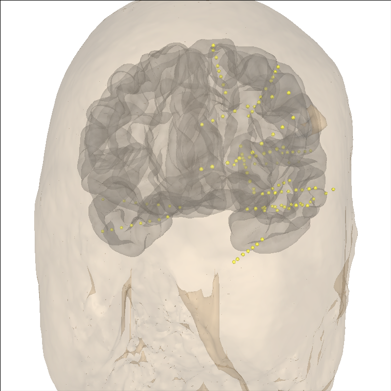
Let’s check to make sure everything is aligned.

Note

The most rostral electrode in the temporal lobe is outside the fsaverage template brain. This is not ideal but it is the best that the linear Talairach transform can accomplish. A more complex transform is necessary for more accurate warping, see Locating intracranial electrode contacts.

# compute the transform to head for plotting
trans = mne.channels.compute_native_head_t(montage)
# note that this is the same as:
# ``mne.transforms.invert_transform(
#      mne.transforms.combine_transforms(head_mri_t, mri_mni_t))``

view_kwargs = dict(azimuth=105, elevation=100, focalpoint=(0, 0, -15))
brain = mne.viz.Brain(
    "fsaverage",
    subjects_dir=subjects_dir,
    cortex="low_contrast",
    alpha=0.25,
    background="white",
)
brain.add_sensors(epochs.info, trans=trans)
brain.add_head(alpha=0.25, color="tan")
brain.show_view(distance=400, **view_kwargs)

Channel types:: seeg: 119
Using fsaverage-head-dense.fif for head surface.
    1 BEM surfaces found
    Reading a surface...
[done]
    1 BEM surfaces read

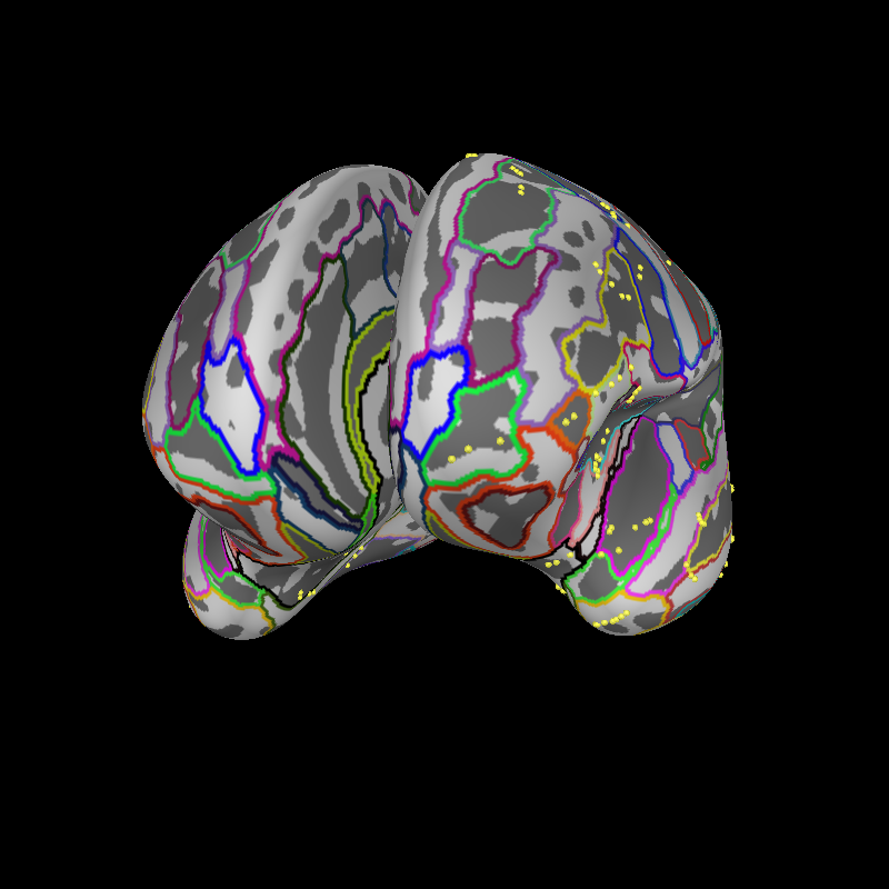
Now, let’s project onto the inflated brain surface for visualization. This video may be helpful for understanding the how the annotations on the pial surface translate to the inflated brain and flat map:

brain = mne.viz.Brain(
    "fsaverage", subjects_dir=subjects_dir, surf="inflated", background="black"
)
brain.add_annotation("aparc.a2009s")
brain.add_sensors(epochs.info, trans=trans)
brain.show_view(distance=500, **view_kwargs)

Channel types:: seeg: 119

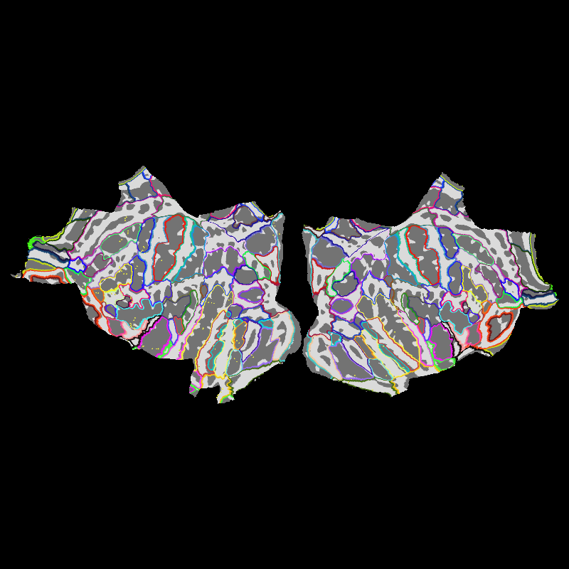
Let’s also show the sensors on a flat brain.

brain = mne.viz.Brain(
    "fsaverage", subjects_dir=subjects_dir, surf="flat", background="black"
)
brain.add_annotation("aparc.a2009s")
brain.add_sensors(epochs.info, trans=trans)

Channel types:: seeg: 119

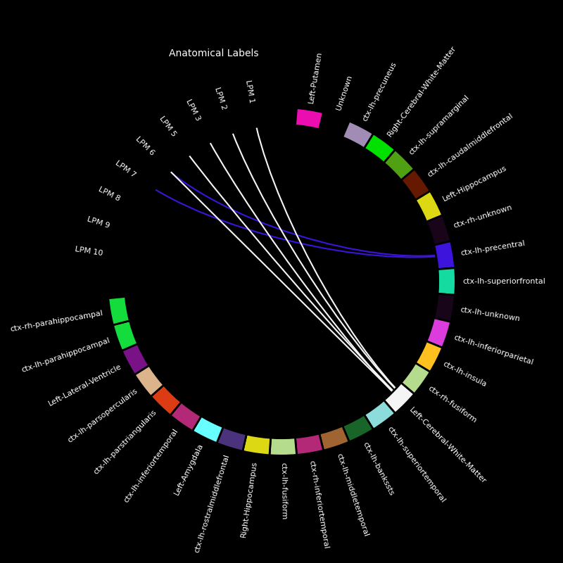
Let’s also look at which regions of interest are nearby our electrode contacts.

aseg = "aparc+aseg"  # parcellation/anatomical segmentation atlas
labels, colors = mne.get_montage_volume_labels(
    montage, "fsaverage", subjects_dir=subjects_dir, aseg=aseg
)

# separate by electrodes which have names like LAMY 1
electrodes = set(
    [
        "".join([lttr for lttr in ch_name if not lttr.isdigit() and lttr != " "])
        for ch_name in montage.ch_names
    ]
)
print(f"Electrodes in the dataset: {electrodes}")

electrodes = ("LPM", "LSMA")  # choose two for this example
for elec in electrodes:
    picks = [ch_name for ch_name in epochs.ch_names if elec in ch_name]
    fig, ax = mne.viz.plot_channel_labels_circle(labels, colors, picks=picks)
    fig.text(0.3, 0.9, "Anatomical Labels", color="white")

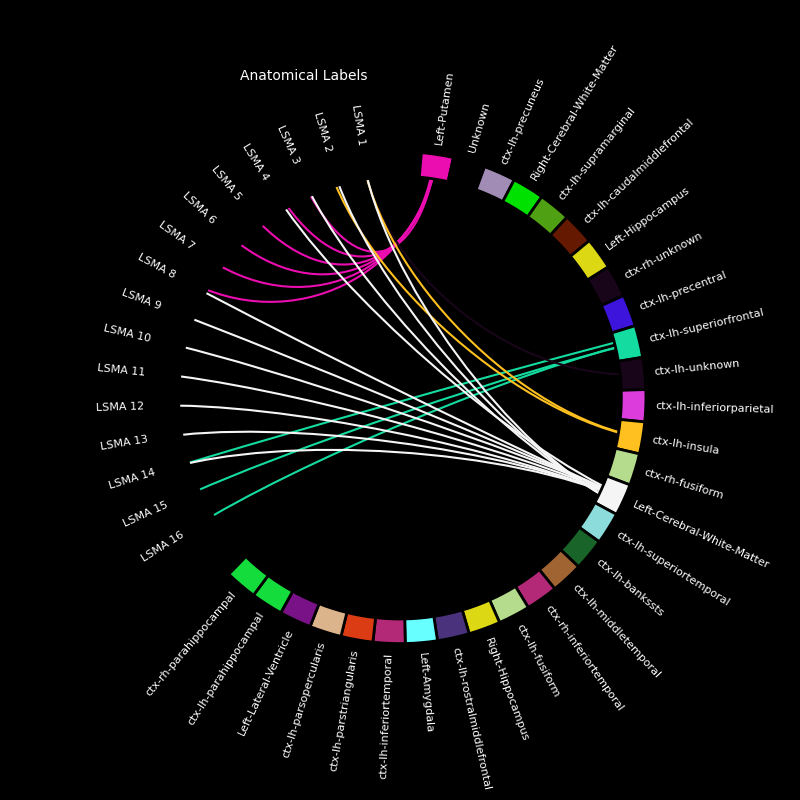
Electrodes in the dataset: {'LPIT', 'LPCN', 'LOFC', 'LTPO', 'LSMA', 'RAHP', 'LSTG', 'LPHG', 'LPLI', 'LBRI', 'LAMY', 'LACN', 'RPHP', 'LENT', 'LPM'}

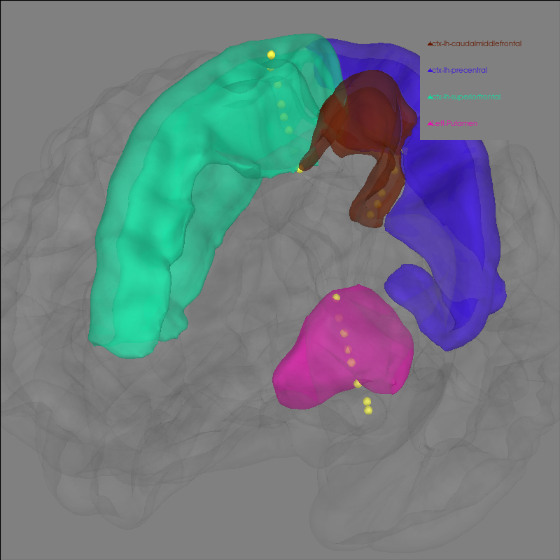
Now, let’s the electrodes and a few regions of interest that the contacts of the electrode are proximal to.

picks = [
    ii
    for ii, ch_name in enumerate(epochs.ch_names)
    if any([elec in ch_name for elec in electrodes])
]
labels = (
    "ctx-lh-caudalmiddlefrontal",
    "ctx-lh-precentral",
    "ctx-lh-superiorfrontal",
    "Left-Putamen",
)

fig = mne.viz.plot_alignment(
    mne.pick_info(epochs.info, picks),
    trans,
    "fsaverage",
    subjects_dir=subjects_dir,
    surfaces=[],
    coord_frame="mri",
)

brain = mne.viz.Brain(
    "fsaverage",
    alpha=0.1,
    cortex="low_contrast",
    subjects_dir=subjects_dir,
    units="m",
    figure=fig,
)
brain.add_volume_labels(aseg="aparc+aseg", labels=labels)
brain.show_view(azimuth=120, elevation=90, distance=0.25)

Channel types:: seeg: 25
    Smoothing by a factor of 0.9

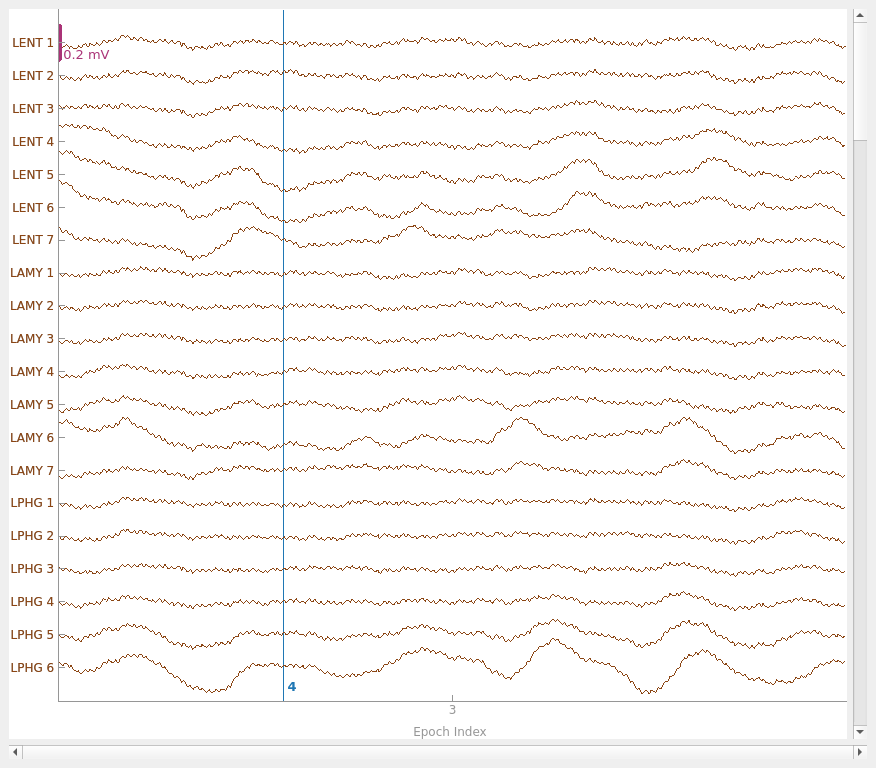
Next, we’ll get the epoch data and plot its amplitude over time.

epochs.plot(events=True)

Loading data for 1 events and 701 original time points ...
0 bad epochs dropped
Loading data for 1 events and 701 original time points ...
Loading data for 1 events and 701 original time points ...

We can visualize this raw data on the fsaverage brain (in MNI space) as a heatmap. This works by first creating an Evoked data structure from the data of interest (in this example, it is just the raw LFP). Then one should generate a stc data structure, which will be able to visualize source activity on the brain in various different formats.

# get standard fsaverage volume (5mm grid) source space
fname_src = subjects_dir / "fsaverage" / "bem" / "fsaverage-vol-5-src.fif"
vol_src = mne.read_source_spaces(fname_src)

evoked = epochs.average()
stc = mne.stc_near_sensors(
    evoked,
    trans,
    "fsaverage",
    subjects_dir=subjects_dir,
    src=vol_src,
    surface=None,
    verbose="error",
)
stc = abs(stc)  # just look at magnitude
clim = dict(kind="value", lims=np.percentile(abs(evoked.data), [10, 50, 75]))

Reading a source space...
[done]
1 source spaces read

Plot 3D source (brain region) visualization:

By default, stc.plot_3d() will show a time course of the source with the largest absolute value across any time point. In this example, it is simply the source with the largest raw signal value. Its location is marked on the brain by a small blue sphere.

brain = stc.plot_3d(
    src=vol_src,
    subjects_dir=subjects_dir,
    view_layout="horizontal",
    views=["axial", "coronal", "sagittal"],
    size=(800, 300),
    show_traces=0.4,
    clim=clim,
    add_data_kwargs=dict(colorbar_kwargs=dict(label_font_size=8)),
)

# You can save a movie like the one on our documentation website with:
# brain.save_movie(time_dilation=3, interpolation='linear', framerate=5,
#                  time_viewer=True, filename='./mne-test-seeg.m4')

In this tutorial, we used a BEM surface for the fsaverage subject from FreeSurfer.

For additional common analyses of interest, see the following:

For volumetric plotting options, including limiting to a specific area of the volume specified by say an atlas, or plotting different types of source visualizations see: Visualize source time courses (stcs).
For extracting activation within a specific FreeSurfer volume and using different FreeSurfer volumes, see: How MNE uses FreeSurfer’s outputs.
For working with BEM surfaces and using FreeSurfer, or MNE to generate them, see: Head model and forward computation.

Total running time of the script: (0 minutes 58.356 seconds)

Estimated memory usage: 583 MB

Gallery generated by Sphinx-Gallery