Note
Go to the end to download the full example code.
Plotting with mne.viz.Brain#
In this example, we’ll show how to use mne.viz.Brain.
# Author: Alex Rockhill <aprockhill@mailbox.org>
#
# License: BSD-3-Clause
# Copyright the MNE-Python contributors.
Load data#
In this example we use the sample data which is data from a subject
being presented auditory and visual stimuli to display the functionality
of mne.viz.Brain for plotting data on a brain.
import matplotlib.pyplot as plt
import numpy as np
from matplotlib.cm import ScalarMappable
from matplotlib.colors import Normalize

import mne
from mne.datasets import sample

print(__doc__)

data_path = sample.data_path()
subjects_dir = data_path / "subjects"
sample_dir = data_path / "MEG" / "sample"
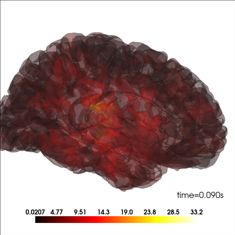
Add source information#
Plot source information.
brain_kwargs = dict(alpha=0.1, background="white", cortex="low_contrast")
brain = mne.viz.Brain("sample", subjects_dir=subjects_dir, **brain_kwargs)

stc = mne.read_source_estimate(sample_dir / "sample_audvis-meg")
stc.crop(0.09, 0.1)

kwargs = dict(
    fmin=stc.data.min(),
    fmax=stc.data.max(),
    alpha=0.25,
    smoothing_steps="nearest",
    time=stc.times,
)
brain.add_data(stc.lh_data, hemi="lh", vertices=stc.lh_vertno, **kwargs)
brain.add_data(stc.rh_data, hemi="rh", vertices=stc.rh_vertno, **kwargs)
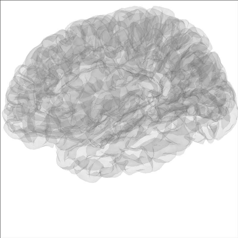
Modify the view of the brain#
You can adjust the view of the brain using show_view method.
brain = mne.viz.Brain("sample", subjects_dir=subjects_dir, **brain_kwargs)
brain.show_view(azimuth=190, elevation=70, distance=350, focalpoint=(0, 0, 20))
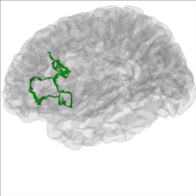
Highlight a region on the brain#
It can be useful to highlight a region of the brain for analyses.
To highlight a region on the brain you can use the add_label method.
Labels are stored in the FreeSurfer label directory from the recon-all
for that subject. Labels can also be made following the
FreeSurfer instructions
Here we will show Brodmann Area 44.
Note
The MNE sample dataset contains only a subselection of the
FreeSurfer labels created during the recon-all.
brain = mne.viz.Brain("sample", subjects_dir=subjects_dir, **brain_kwargs)
brain.add_label("BA44", hemi="lh", color="green", borders=True)
brain.show_view(azimuth=190, elevation=70, distance=350, focalpoint=(0, 0, 20))
Include the head in the image#
Add a head image using the add_head method.
brain = mne.viz.Brain("sample", subjects_dir=subjects_dir, **brain_kwargs)
brain.add_head(alpha=0.5)
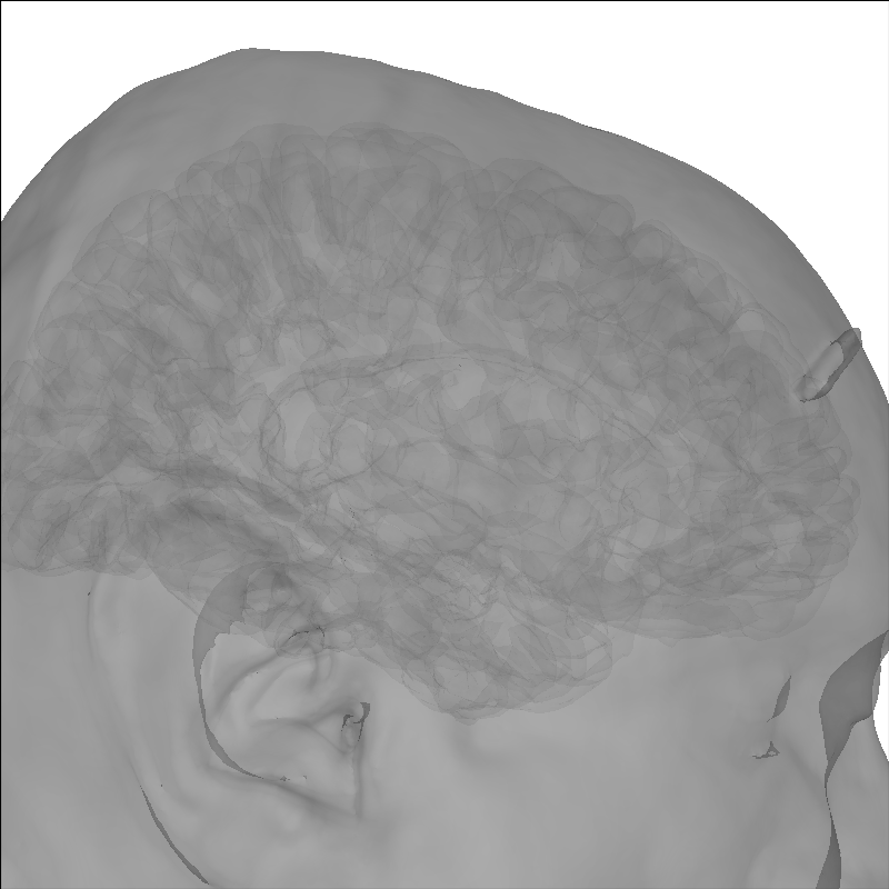
Using lh.seghead for head surface.
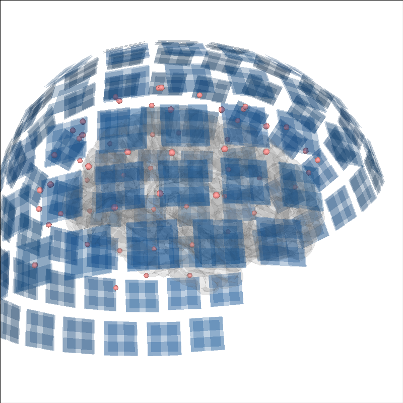
Add sensors positions#
To put into context the data that generated the source time course, the sensor positions can be displayed as well.
brain = mne.viz.Brain("sample", subjects_dir=subjects_dir, **brain_kwargs)
evoked = mne.read_evokeds(sample_dir / "sample_audvis-ave.fif")[0]
trans = mne.read_trans(sample_dir / "sample_audvis_raw-trans.fif")
brain.add_sensors(evoked.info, trans)
brain.show_view(distance=500)  # move back to show sensors
Reading /home/circleci/mne_data/MNE-sample-data/MEG/sample/sample_audvis-ave.fif ...
    Read a total of 4 projection items:
        PCA-v1 (1 x 10²) active
        PCA-v2 (1 x 10²) active
        PCA-v3 (1 x 10²) active
        Average EEG reference (1 x 60) active
    Found the data of interest:
        t =    -199.80 ...     499.49 ms (Left Auditory)
        0 CTF compensation matrices available
        nave = 55 - aspect type = 100
Projections have already been applied. Setting proj attribute to True.
No baseline correction applied
    Read a total of 4 projection items:
        PCA-v1 (1 x 10²) active
        PCA-v2 (1 x 10²) active
        PCA-v3 (1 x 10²) active
        Average EEG reference (1 x 60) active
    Found the data of interest:
        t =    -199.80 ...     499.49 ms (Right Auditory)
        0 CTF compensation matrices available
        nave = 61 - aspect type = 100
Projections have already been applied. Setting proj attribute to True.
No baseline correction applied
    Read a total of 4 projection items:
        PCA-v1 (1 x 10²) active
        PCA-v2 (1 x 10²) active
        PCA-v3 (1 x 10²) active
        Average EEG reference (1 x 60) active
    Found the data of interest:
        t =    -199.80 ...     499.49 ms (Left visual)
        0 CTF compensation matrices available
        nave = 67 - aspect type = 100
Projections have already been applied. Setting proj attribute to True.
No baseline correction applied
    Read a total of 4 projection items:
        PCA-v1 (1 x 10²) active
        PCA-v2 (1 x 10²) active
        PCA-v3 (1 x 10²) active
        Average EEG reference (1 x 60) active
    Found the data of interest:
        t =    -199.80 ...     499.49 ms (Right visual)
        0 CTF compensation matrices available
        nave = 58 - aspect type = 100
Projections have already been applied. Setting proj attribute to True.
No baseline correction applied
Channel types:: grad: 203, mag: 102, eeg: 59
Getting helmet for system 306m
Add current dipoles#
Dipole modeling as in The role of dipole orientations in distributed source localization can be plotted on the brain as well.
brain = mne.viz.Brain("sample", subjects_dir=subjects_dir, **brain_kwargs)
dip = mne.read_dipole(sample_dir / "sample_audvis_set1.dip")
cmap = plt.colormaps["YlOrRd"]
colors = [cmap(gof / dip.gof.max()) for gof in dip.gof]
brain.add_dipole(dip, trans, colors=colors, scales=list(dip.amplitude * 1e8))
brain.show_view(azimuth=-20, elevation=60, distance=300)
img = brain.screenshot()  # for next section
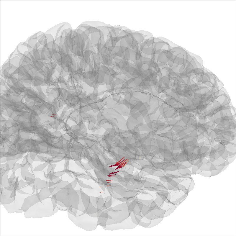
34 dipole(s) found
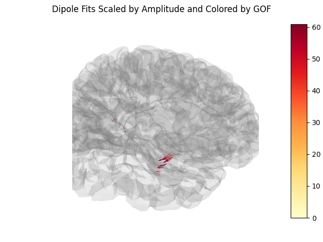
Create a screenshot for exporting the brain image#
Also, we can a static image of the brain using screenshot (above),
which will allow us to add a colorbar. This is useful for figures in
publications.
fig, ax = plt.subplots()
ax.imshow(img)
ax.axis("off")
cax = fig.add_axes([0.9, 0.1, 0.05, 0.8])
norm = Normalize(vmin=0, vmax=dip.gof.max())
fig.colorbar(ScalarMappable(norm=norm, cmap=cmap), cax=cax)
fig.suptitle("Dipole Fits Scaled by Amplitude and Colored by GOF")
Update overlays via Brain.layered_meshes#
After add_data() is called, each hemisphere’s surface
is backed by a LayeredMesh stored in
brain.layered_meshes. Calling
update_overlay() pushes new scalar data without
rebuilding the full rendering pipeline — the key operation for packages that
stream source-space data onto the brain in real time, such as
MNE-RT.
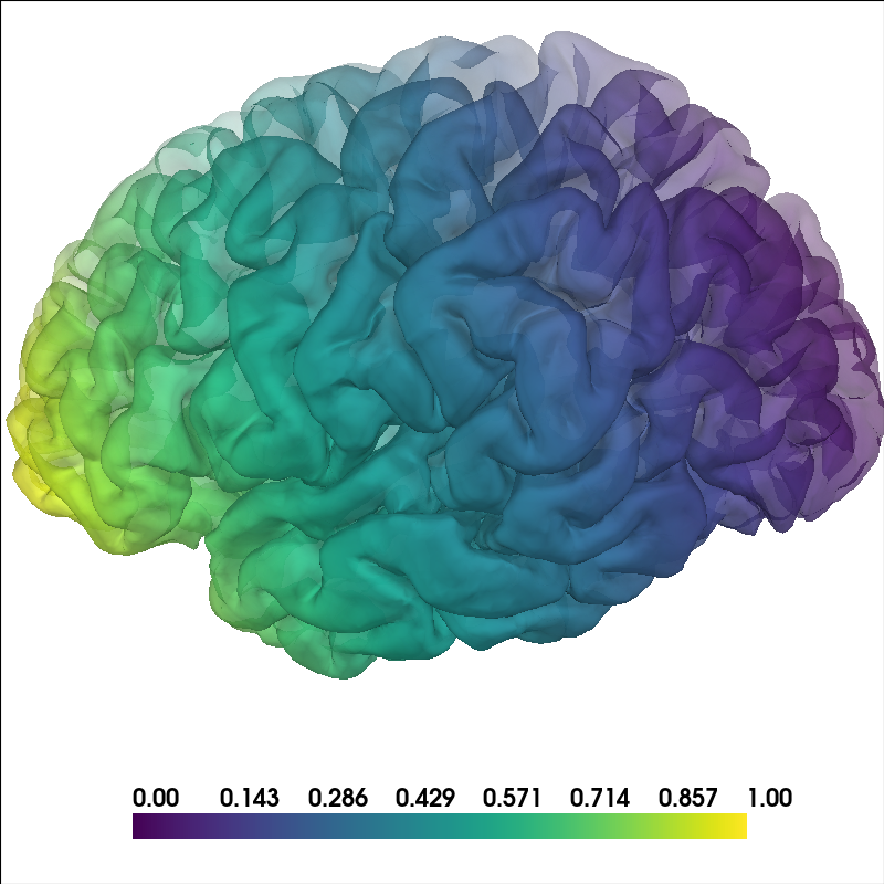
Here we add an initial bottom-to-top gradient as the first data frame.
brain = mne.viz.Brain("sample", subjects_dir=subjects_dir, hemi="lh", **brain_kwargs)
coords = brain.geo["lh"].coords
data_t0 = coords[:, 2]
data_t0 = (data_t0 - data_t0.min()) / (data_t0.max() - data_t0.min())
brain.add_data(
    data_t0, hemi="lh", fmin=0, fmax=1, colormap="viridis", smoothing_steps=5
)
brain.show_view(azimuth=190, elevation=70, distance=350, focalpoint=(0, 0, 20))

Simulate a new data frame arriving: call
update_overlay() on the same brain to replace
the scalars in-place — no new mesh, no new actor, no pipeline rebuild.
# we create a new brain here for comparison purposes
brain_update = mne.viz.Brain(
    "sample", subjects_dir=subjects_dir, hemi="lh", **brain_kwargs
)
brain_update.add_data(
    data_t0, hemi="lh", fmin=0, fmax=1, colormap="viridis", smoothing_steps=5
)
brain_update.show_view(azimuth=190, elevation=70, distance=350, focalpoint=(0, 0, 20))
data_t1 = coords[:, 1]
data_t1 = (data_t1 - data_t1.min()) / (data_t1.max() - data_t1.min())
mesh = brain_update.layered_meshes["lh"]
mesh.update_overlay(name="data", scalars=data_t1)
mesh.update()
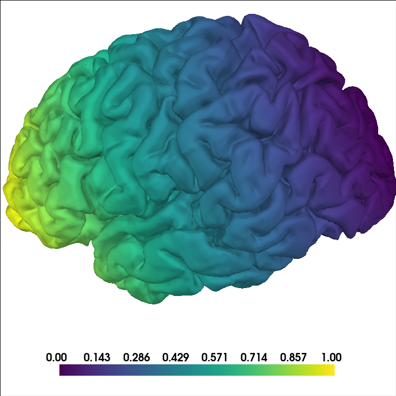
Use per-vertex opacity for distributed data#
You can provide an array for alpha in mne.viz.Brain.add_data()
to control transparency per vertex. This can be useful to emphasize a
subset of vertices while still showing surrounding context.
brain = mne.viz.Brain("sample", subjects_dir=subjects_dir, hemi="lh", **brain_kwargs)
coords = brain.geo["lh"].coords
n_vertices = len(coords)

# Build synthetic data: a smooth left-to-right gradient color-wise in the Y
# (front-back) direction, plus a matching opacity ramp from mostly transparent to
# fully opaque in the X (left-right) direction.
data = coords[:, 1]
data = (data - data.min()) / (data.max() - data.min())
vertex_alpha = -coords[:, 0]
vertex_alpha = (vertex_alpha - vertex_alpha.min()) / (
    vertex_alpha.max() - vertex_alpha.min()
)

brain.add_data(
    data,
    hemi="lh",
    alpha=vertex_alpha,
    colormap="viridis",
    smoothing_steps=5,
)
brain.show_view(azimuth=190, elevation=70, distance=350, focalpoint=(0, 0, 20))
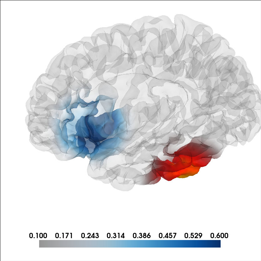
Composite two overlays simultaneously#
Pass remove_existing=False and a distinct key to keep the first
overlay visible while adding a second one on top. The two layers are
alpha-composited by LayeredMesh so both datasets appear
at the same time.
Here we simulate two focal patches of activity evolving over time in different brain regions: a temporal source (red/hot) that peaks early and a frontal source (blue) that peaks later. In the interactive viewer an “Overlay” drop-down appears in the Color Limits panel — use it to switch which overlay’s limits and smoothing the sliders control.
brain = mne.viz.Brain(
    "sample",
    subjects_dir=subjects_dir,
    hemi="lh",
    alpha=0.1,
    background="white",
    cortex="low_contrast",
)
coords = brain.geo["lh"].coords  # vertex positions in mm


def gaussian_patch(coords, center, sigma=15.0):
    """Gaussian blob of activity centred on a surface coordinate (mm)."""
    d = np.linalg.norm(coords - center, axis=1)
    return np.exp(-(d**2) / (2 * sigma**2))


temporal = gaussian_patch(coords, center=np.array([-52.0, -18.0, -8.0]))
brain.add_data(
    temporal,
    hemi="lh",
    fmin=0.1,
    fmax=1.5,
    colormap="hot",
    transparent=True,
    key="temporal",
    smoothing_steps=5,
)

frontal = gaussian_patch(coords, center=np.array([-38.0, 28.0, 46.0]))
brain.add_data(
    frontal,
    hemi="lh",
    fmin=0.1,
    fmax=0.6,
    colormap="Blues",
    transparent=True,
    alpha=0.5,
    key="frontal",
    remove_existing=False,
    smoothing_steps=5,
)
brain.show_view(azimuth=180, elevation=70, distance=380, focalpoint=(0, 10, 20))
Total running time of the script: (1 minutes 5.797 seconds)