Note
Go to the end to download the full example code.
Mass-univariate twoway repeated measures ANOVA on single trial power#
This script shows how to conduct a mass-univariate repeated measures ANOVA. As the model to be fitted assumes two fully crossed factors, we will study the interplay between perceptual modality (auditory VS visual) and the location of stimulus presentation (left VS right). Here we use single trials as replications (subjects) while iterating over time slices plus frequency bands for to fit our mass-univariate model. For the sake of simplicity we will confine this analysis to one single channel of which we know that it exposes a strong induced response. We will then visualize each effect by creating a corresponding mass-univariate effect image. We conclude with accounting for multiple comparisons by performing a permutation clustering test using the ANOVA as clustering function. The results final will be compared to multiple comparisons using False Discovery Rate correction.
# Authors: Denis Engemann <denis.engemann@gmail.com>
#          Eric Larson <larson.eric.d@gmail.com>
#          Alexandre Gramfort <alexandre.gramfort@inria.fr>
#          Alex Rockhill <aprockhill@mailbox.org>
#
# License: BSD-3-Clause
# Copyright the MNE-Python contributors.
import matplotlib.pyplot as plt
import numpy as np

import mne
from mne.datasets import sample
from mne.stats import f_mway_rm, f_threshold_mway_rm, fdr_correction

print(__doc__)
Set parameters#
data_path = sample.data_path()
meg_path = data_path / "MEG" / "sample"
raw_fname = meg_path / "sample_audvis_raw.fif"
event_fname = meg_path / "sample_audvis_raw-eve.fif"
tmin, tmax = -0.2, 0.5

# Setup for reading the raw data
raw = mne.io.read_raw_fif(raw_fname)
events = mne.read_events(event_fname)

include = []
raw.info["bads"] += ["MEG 2443"]  # bads

# picks MEG gradiometers
picks = mne.pick_types(
    raw.info,
    meg="grad",
    eeg=False,
    eog=True,
    stim=False,
    include=include,
    exclude="bads",
)

ch_name = "MEG 1332"

# Load conditions
reject = dict(grad=4000e-13, eog=150e-6)
event_id = dict(aud_l=1, aud_r=2, vis_l=3, vis_r=4)
epochs = mne.Epochs(
    raw,
    events,
    event_id,
    tmin,
    tmax,
    picks=picks,
    baseline=(None, 0),
    preload=True,
    reject=reject,
)
epochs.pick([ch_name])  # restrict example to one channel
Opening raw data file /home/circleci/mne_data/MNE-sample-data/MEG/sample/sample_audvis_raw.fif...
    Read a total of 3 projection items:
        PCA-v1 (1 x 10²)  idle
        PCA-v2 (1 x 10²)  idle
        PCA-v3 (1 x 10²)  idle
    Range : 25800 ... 192599 =     42.956 ...   320.670 secs
Ready.
Not setting metadata
289 matching events found
Setting baseline interval to [-0.19979521315838786, 0.0] s
Applying baseline correction (mode: mean)
0 projection items activated
Loading data for 289 events and 421 original time points ...
    Rejecting  epoch based on EOG : ['EOG 061']
    Rejecting  epoch based on EOG : ['EOG 061']
    Rejecting  epoch based on EOG : ['EOG 061']
    Rejecting  epoch based on EOG : ['EOG 061']
    Rejecting  epoch based on EOG : ['EOG 061']
    Rejecting  epoch based on EOG : ['EOG 061']
    Rejecting  epoch based on EOG : ['EOG 061']
    Rejecting  epoch based on EOG : ['EOG 061']
    Rejecting  epoch based on EOG : ['EOG 061']
    Rejecting  epoch based on EOG : ['EOG 061']
    Rejecting  epoch based on EOG : ['EOG 061']
    Rejecting  epoch based on EOG : ['EOG 061']
    Rejecting  epoch based on EOG : ['EOG 061']
    Rejecting  epoch based on EOG : ['EOG 061']
    Rejecting  epoch based on EOG : ['EOG 061']
    Rejecting  epoch based on EOG : ['EOG 061']
    Rejecting  epoch based on EOG : ['EOG 061']
    Rejecting  epoch based on EOG : ['EOG 061']
    Rejecting  epoch based on EOG : ['EOG 061']
    Rejecting  epoch based on EOG : ['EOG 061']
    Rejecting  epoch based on EOG : ['EOG 061']
    Rejecting  epoch based on EOG : ['EOG 061']
    Rejecting  epoch based on EOG : ['EOG 061']
    Rejecting  epoch based on EOG : ['EOG 061']
    Rejecting  epoch based on EOG : ['EOG 061']
    Rejecting  epoch based on EOG : ['EOG 061']
    Rejecting  epoch based on EOG : ['EOG 061']
    Rejecting  epoch based on EOG : ['EOG 061']
    Rejecting  epoch based on EOG : ['EOG 061']
    Rejecting  epoch based on EOG : ['EOG 061']
    Rejecting  epoch based on EOG : ['EOG 061']
    Rejecting  epoch based on EOG : ['EOG 061']
    Rejecting  epoch based on EOG : ['EOG 061']
    Rejecting  epoch based on EOG : ['EOG 061']
    Rejecting  epoch based on EOG : ['EOG 061']
    Rejecting  epoch based on EOG : ['EOG 061']
    Rejecting  epoch based on EOG : ['EOG 061']
    Rejecting  epoch based on EOG : ['EOG 061']
    Rejecting  epoch based on EOG : ['EOG 061']
    Rejecting  epoch based on EOG : ['EOG 061']
    Rejecting  epoch based on EOG : ['EOG 061']
    Rejecting  epoch based on EOG : ['EOG 061']
    Rejecting  epoch based on EOG : ['EOG 061']
    Rejecting  epoch based on EOG : ['EOG 061']
    Rejecting  epoch based on EOG : ['EOG 061']
    Rejecting  epoch based on EOG : ['EOG 061']
    Rejecting  epoch based on EOG : ['EOG 061']
    Rejecting  epoch based on EOG : ['EOG 061']
    Rejecting  epoch based on EOG : ['EOG 061']
    Rejecting  epoch based on EOG : ['EOG 061']
    Rejecting  epoch based on EOG : ['EOG 061']
    Rejecting  epoch based on EOG : ['EOG 061']
    Rejecting  epoch based on EOG : ['EOG 061']
53 bad epochs dropped
We have to make sure all conditions have the same counts, as the ANOVA expects a fully balanced data matrix and does not forgive imbalances that generously (risk of type-I error).
epochs.equalize_event_counts(event_id)

# Factor to down-sample the temporal dimension of the TFR computed by
# tfr_morlet.
decim = 2
freqs = np.arange(7, 30, 3)  # define frequencies of interest
n_cycles = freqs / freqs[0]
zero_mean = False  # don't correct morlet wavelet to be of mean zero
# To have a true wavelet zero_mean should be True but here for illustration
# purposes it helps to spot the evoked response.
Dropped 12 epochs: 50, 92, 128, 147, 152, 154, 155, 186, 196, 198, 206, 207
Create TFR representations for all conditions#
epochs_power = list()
for condition in [epochs[k] for k in event_id]:
    this_tfr = condition.compute_tfr(
        "morlet",
        freqs,
        n_cycles=n_cycles,
        decim=decim,
        average=False,
        zero_mean=zero_mean,
        return_itc=False,
    )
    this_tfr.apply_baseline(mode="ratio", baseline=(None, 0))
    this_power = this_tfr.data[:, 0, :, :]  # we only have one channel.
    epochs_power.append(this_power)
Applying baseline correction (mode: ratio)
Applying baseline correction (mode: ratio)
Applying baseline correction (mode: ratio)
Applying baseline correction (mode: ratio)
Setup repeated measures ANOVA#
We will tell the ANOVA how to interpret the data matrix in terms of factors. This is done via the factor levels argument which is a list of the number factor levels for each factor.
n_conditions = len(epochs.event_id)
n_replications = epochs.events.shape[0] // n_conditions

factor_levels = [2, 2]  # number of levels in each factor
effects = "A*B"  # this is the default signature for computing all effects
# Other possible options are 'A' or 'B' for the corresponding main effects
# or 'A:B' for the interaction effect only (this notation is borrowed from the
# R formula language)
n_freqs = len(freqs)
times = 1e3 * epochs.times[::decim]
n_times = len(times)
Now we’ll assemble the data matrix and swap axes so the trial replications are the first dimension and the conditions are the second dimension.
data = np.swapaxes(np.asarray(epochs_power), 1, 0)

# so we have replications × conditions × observations
# where the time-frequency observations are freqs × times:
print(data.shape)
(56, 4, 8, 211)
While the iteration scheme used above for assembling the data matrix makes sure the first two dimensions are organized as expected (with A = modality and B = location):
trial |
A1B1 |
A1B2 |
A2B1 |
B2B2 |
|---|---|---|---|---|
1 |
1.34 |
2.53 |
0.97 |
1.74 |
… |
… |
… |
… |
… |
56 |
2.45 |
7.90 |
3.09 |
4.76 |
Now we’re ready to run our repeated measures ANOVA.
Note. As we treat trials as subjects, the test only accounts for time locked responses despite the ‘induced’ approach. For analysis for induced power at the group level averaged TRFs are required.
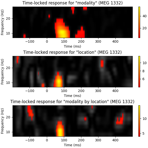
fvals, pvals = f_mway_rm(data, factor_levels, effects=effects)

effect_labels = ["modality", "location", "modality by location"]

fig, axes = plt.subplots(3, 1, figsize=(6, 6), layout="constrained")

# let's visualize our effects by computing f-images
for effect, sig, effect_label, ax in zip(fvals, pvals, effect_labels, axes):
    # show naive F-values in gray
    ax.imshow(
        effect,
        cmap="gray",
        aspect="auto",
        origin="lower",
        extent=[times[0], times[-1], freqs[0], freqs[-1]],
    )
    # create mask for significant time-frequency locations
    effect[sig >= 0.05] = np.nan
    c = ax.imshow(
        effect,
        cmap="autumn",
        aspect="auto",
        origin="lower",
        extent=[times[0], times[-1], freqs[0], freqs[-1]],
    )
    fig.colorbar(c, ax=ax)
    ax.set_xlabel("Time (ms)")
    ax.set_ylabel("Frequency (Hz)")
    ax.set_title(f'Time-locked response for "{effect_label}" ({ch_name})')
Account for multiple comparisons using FDR versus permutation clustering test#
First we need to slightly modify the ANOVA function to be suitable for the clustering procedure. Also want to set some defaults. Let’s first override effects to confine the analysis to the interaction
effects = "A:B"
A stat_fun must deal with a variable number of input arguments. Inside the clustering function each condition will be passed as flattened array, necessitated by the clustering procedure. The ANOVA however expects an input array of dimensions: subjects × conditions × observations (optional). The following function catches the list input and swaps the first and the second dimension and finally calls the ANOVA function.
def stat_fun(*args):
    return f_mway_rm(
        np.swapaxes(args, 1, 0),
        factor_levels=factor_levels,
        effects=effects,
        return_pvals=False,
    )[0]


# The ANOVA returns a tuple f-values and p-values, we will pick the former.
pthresh = 0.001  # set threshold rather high to save some time
f_thresh = f_threshold_mway_rm(n_replications, factor_levels, effects, pthresh)
tail = 1  # f-test, so tail > 0
n_permutations = 256  # Save some time (the test won't be too sensitive ...)
F_obs, clusters, cluster_p_values, h0 = mne.stats.permutation_cluster_test(
    epochs_power,
    stat_fun=stat_fun,
    threshold=f_thresh,
    tail=tail,
    n_jobs=None,
    n_permutations=n_permutations,
    buffer_size=None,
    out_type="mask",
    seed=0,
)
stat_fun(H1): min=6.658469887778116e-07 max=14.419588379647625
Running initial clustering …
Found 1 cluster

  0%|          | Permuting : 0/255 [00:00<?,       ?it/s]
  0%|          | Permuting : 1/255 [00:00<00:08,   29.42it/s]
  1%|          | Permuting : 2/255 [00:00<00:08,   29.52it/s]
  2%|▏         | Permuting : 4/255 [00:00<00:06,   39.94it/s]
  2%|▏         | Permuting : 6/255 [00:00<00:05,   45.13it/s]
  3%|▎         | Permuting : 7/255 [00:00<00:05,   41.69it/s]
  4%|▎         | Permuting : 9/255 [00:00<00:05,   45.00it/s]
  4%|▍         | Permuting : 11/255 [00:00<00:05,   47.36it/s]
  5%|▍         | Permuting : 12/255 [00:00<00:05,   44.73it/s]
  5%|▌         | Permuting : 14/255 [00:00<00:05,   46.69it/s]
  6%|▌         | Permuting : 15/255 [00:00<00:05,   44.55it/s]
  7%|▋         | Permuting : 17/255 [00:00<00:05,   46.25it/s]
  7%|▋         | Permuting : 18/255 [00:00<00:05,   44.45it/s]
  8%|▊         | Permuting : 20/255 [00:00<00:05,   45.98it/s]
  9%|▊         | Permuting : 22/255 [00:00<00:04,   47.26it/s]
  9%|▉         | Permuting : 23/255 [00:00<00:05,   45.62it/s]
 10%|▉         | Permuting : 25/255 [00:00<00:04,   46.84it/s]
 10%|█         | Permuting : 26/255 [00:00<00:05,   45.37it/s]
 11%|█         | Permuting : 28/255 [00:00<00:04,   46.52it/s]
 11%|█▏        | Permuting : 29/255 [00:00<00:05,   45.17it/s]
 12%|█▏        | Permuting : 31/255 [00:00<00:04,   46.27it/s]
 13%|█▎        | Permuting : 32/255 [00:00<00:04,   45.01it/s]
 13%|█▎        | Permuting : 34/255 [00:00<00:04,   46.06it/s]
 14%|█▍        | Permuting : 36/255 [00:00<00:04,   47.01it/s]
 15%|█▍        | Permuting : 37/255 [00:00<00:04,   45.78it/s]
 15%|█▌        | Permuting : 39/255 [00:00<00:04,   46.70it/s]
 16%|█▌        | Permuting : 40/255 [00:00<00:04,   45.54it/s]
 16%|█▋        | Permuting : 42/255 [00:00<00:04,   46.45it/s]
 17%|█▋        | Permuting : 43/255 [00:00<00:04,   45.35it/s]
 18%|█▊        | Permuting : 45/255 [00:00<00:04,   46.25it/s]
 18%|█▊        | Permuting : 46/255 [00:01<00:04,   45.19it/s]
 19%|█▉        | Permuting : 48/255 [00:01<00:04,   46.06it/s]
 19%|█▉        | Permuting : 49/255 [00:01<00:04,   45.04it/s]
 20%|██        | Permuting : 51/255 [00:01<00:04,   45.91it/s]
 21%|██        | Permuting : 53/255 [00:01<00:04,   46.70it/s]
 21%|██        | Permuting : 54/255 [00:01<00:04,   45.68it/s]
 22%|██▏       | Permuting : 56/255 [00:01<00:04,   46.48it/s]
 22%|██▏       | Permuting : 57/255 [00:01<00:04,   45.49it/s]
 23%|██▎       | Permuting : 59/255 [00:01<00:04,   46.29it/s]
 24%|██▎       | Permuting : 60/255 [00:01<00:04,   45.33it/s]
 24%|██▍       | Permuting : 62/255 [00:01<00:04,   46.13it/s]
 25%|██▍       | Permuting : 63/255 [00:01<00:04,   45.19it/s]
 25%|██▌       | Permuting : 65/255 [00:01<00:04,   45.98it/s]
 26%|██▌       | Permuting : 66/255 [00:01<00:04,   45.06it/s]
 27%|██▋       | Permuting : 68/255 [00:01<00:04,   45.85it/s]
 27%|██▋       | Permuting : 69/255 [00:01<00:04,   44.95it/s]
 28%|██▊       | Permuting : 71/255 [00:01<00:04,   45.74it/s]
 28%|██▊       | Permuting : 72/255 [00:01<00:04,   44.85it/s]
 29%|██▉       | Permuting : 74/255 [00:01<00:03,   45.64it/s]
 30%|██▉       | Permuting : 76/255 [00:01<00:03,   46.38it/s]
 30%|███       | Permuting : 77/255 [00:01<00:03,   45.47it/s]
 31%|███       | Permuting : 79/255 [00:01<00:03,   46.21it/s]
 31%|███▏      | Permuting : 80/255 [00:01<00:03,   45.32it/s]
 32%|███▏      | Permuting : 82/255 [00:01<00:03,   46.06it/s]
 33%|███▎      | Permuting : 85/255 [00:01<00:03,   48.34it/s]
 34%|███▍      | Permuting : 87/255 [00:01<00:03,   48.92it/s]
 35%|███▌      | Permuting : 90/255 [00:01<00:03,   51.04it/s]
 36%|███▋      | Permuting : 93/255 [00:01<00:03,   53.04it/s]
 37%|███▋      | Permuting : 95/255 [00:01<00:02,   53.36it/s]
 38%|███▊      | Permuting : 98/255 [00:01<00:02,   55.22it/s]
 40%|███▉      | Permuting : 101/255 [00:02<00:02,   56.98it/s]
 40%|████      | Permuting : 103/255 [00:02<00:02,   57.10it/s]
 42%|████▏     | Permuting : 106/255 [00:02<00:02,   58.75it/s]
 42%|████▏     | Permuting : 108/255 [00:02<00:02,   58.78it/s]
 44%|████▎     | Permuting : 111/255 [00:02<00:02,   60.34it/s]
 45%|████▍     | Permuting : 114/255 [00:02<00:02,   61.83it/s]
 46%|████▌     | Permuting : 117/255 [00:02<00:02,   63.23it/s]
 47%|████▋     | Permuting : 119/255 [00:02<00:02,   63.04it/s]
 48%|████▊     | Permuting : 122/255 [00:02<00:02,   64.38it/s]
 49%|████▉     | Permuting : 125/255 [00:02<00:01,   65.65it/s]
 50%|█████     | Permuting : 128/255 [00:02<00:01,   66.85it/s]
 51%|█████▏    | Permuting : 131/255 [00:02<00:01,   67.99it/s]
 52%|█████▏    | Permuting : 133/255 [00:02<00:01,   67.55it/s]
 53%|█████▎    | Permuting : 136/255 [00:02<00:01,   68.65it/s]
 55%|█████▍    | Permuting : 139/255 [00:02<00:01,   69.70it/s]
 56%|█████▌    | Permuting : 142/255 [00:02<00:01,   70.69it/s]
 57%|█████▋    | Permuting : 145/255 [00:02<00:01,   71.63it/s]
 58%|█████▊    | Permuting : 148/255 [00:02<00:01,   72.51it/s]
 59%|█████▉    | Permuting : 150/255 [00:02<00:01,   71.85it/s]
 60%|██████    | Permuting : 153/255 [00:02<00:01,   72.72it/s]
 61%|██████    | Permuting : 156/255 [00:02<00:01,   73.55it/s]
 62%|██████▏   | Permuting : 159/255 [00:02<00:01,   74.34it/s]
 64%|██████▎   | Permuting : 162/255 [00:02<00:01,   75.09it/s]
 65%|██████▍   | Permuting : 165/255 [00:02<00:01,   75.80it/s]
 66%|██████▌   | Permuting : 168/255 [00:02<00:01,   76.47it/s]
 67%|██████▋   | Permuting : 170/255 [00:02<00:01,   75.60it/s]
 68%|██████▊   | Permuting : 173/255 [00:02<00:01,   76.29it/s]
 69%|██████▉   | Permuting : 176/255 [00:02<00:01,   76.94it/s]
 70%|███████   | Permuting : 179/255 [00:02<00:00,   77.56it/s]
 71%|███████▏  | Permuting : 182/255 [00:03<00:00,   78.15it/s]
 73%|███████▎  | Permuting : 185/255 [00:03<00:00,   78.71it/s]
 74%|███████▎  | Permuting : 188/255 [00:03<00:00,   79.24it/s]
 75%|███████▍  | Permuting : 190/255 [00:03<00:00,   78.24it/s]
 76%|███████▌  | Permuting : 193/255 [00:03<00:00,   78.80it/s]
 77%|███████▋  | Permuting : 196/255 [00:03<00:00,   79.32it/s]
 78%|███████▊  | Permuting : 199/255 [00:03<00:00,   79.82it/s]
 79%|███████▉  | Permuting : 202/255 [00:03<00:00,   80.29it/s]
 80%|████████  | Permuting : 205/255 [00:03<00:00,   80.73it/s]
 82%|████████▏ | Permuting : 208/255 [00:03<00:00,   81.15it/s]
 83%|████████▎ | Permuting : 211/255 [00:03<00:00,   81.55it/s]
 84%|████████▍ | Permuting : 214/255 [00:03<00:00,   81.94it/s]
 85%|████████▍ | Permuting : 216/255 [00:03<00:00,   80.81it/s]
 86%|████████▌ | Permuting : 219/255 [00:03<00:00,   81.23it/s]
 87%|████████▋ | Permuting : 222/255 [00:03<00:00,   81.63it/s]
 88%|████████▊ | Permuting : 225/255 [00:03<00:00,   82.01it/s]
 89%|████████▉ | Permuting : 228/255 [00:03<00:00,   82.38it/s]
 91%|█████████ | Permuting : 231/255 [00:03<00:00,   82.72it/s]
 92%|█████████▏| Permuting : 234/255 [00:03<00:00,   83.05it/s]
 93%|█████████▎| Permuting : 237/255 [00:03<00:00,   83.36it/s]
 94%|█████████▍| Permuting : 240/255 [00:03<00:00,   83.66it/s]
 95%|█████████▌| Permuting : 243/255 [00:03<00:00,   83.94it/s]
 96%|█████████▌| Permuting : 245/255 [00:03<00:00,   82.72it/s]
 97%|█████████▋| Permuting : 248/255 [00:03<00:00,   83.04it/s]
 98%|█████████▊| Permuting : 251/255 [00:03<00:00,   83.34it/s]
100%|█████████▉| Permuting : 254/255 [00:03<00:00,   83.63it/s]
100%|██████████| Permuting : 255/255 [00:03<00:00,   66.22it/s]
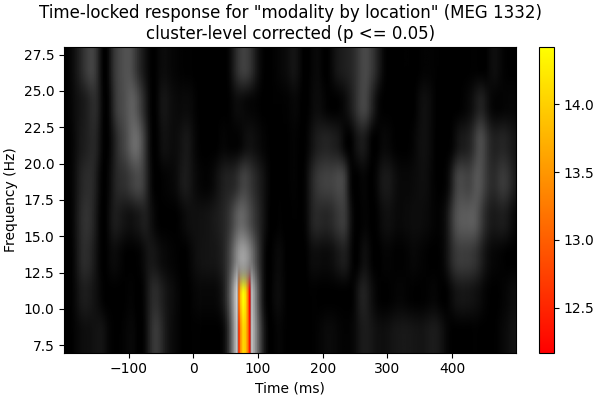
Create new stats image with only significant clusters:
good_clusters = np.where(cluster_p_values < 0.05)[0]
F_obs_plot = np.full_like(F_obs, np.nan)
for ii in good_clusters:
    F_obs_plot[clusters[ii]] = F_obs[clusters[ii]]

fig, ax = plt.subplots(figsize=(6, 4), layout="constrained")
for f_image, cmap in zip([F_obs, F_obs_plot], ["gray", "autumn"]):
    c = ax.imshow(
        f_image,
        cmap=cmap,
        aspect="auto",
        origin="lower",
        extent=[times[0], times[-1], freqs[0], freqs[-1]],
    )

fig.colorbar(c, ax=ax)
ax.set_xlabel("Time (ms)")
ax.set_ylabel("Frequency (Hz)")
ax.set_title(
    f'Time-locked response for "modality by location" ({ch_name})\n'
    "cluster-level corrected (p <= 0.05)"
)
Now using FDR:
mask, _ = fdr_correction(pvals[2])
F_obs_plot2 = F_obs.copy()
F_obs_plot2[~mask.reshape(F_obs_plot.shape)] = np.nan

fig, ax = plt.subplots(figsize=(6, 4), layout="constrained")
for f_image, cmap in zip([F_obs, F_obs_plot2], ["gray", "autumn"]):
    c = ax.imshow(
        f_image,
        cmap=cmap,
        aspect="auto",
        origin="lower",
        extent=[times[0], times[-1], freqs[0], freqs[-1]],
    )

fig.colorbar(c, ax=ax)
ax.set_xlabel("Time (ms)")
ax.set_ylabel("Frequency (Hz)")
ax.set_title(
    f'Time-locked response for "modality by location" ({ch_name})\n'
    "FDR corrected (p <= 0.05)"
)
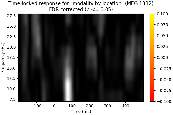
Both cluster-level and FDR correction help get rid of potential false-positives that we saw in the naive f-images. The cluster permutation correction is biased toward time-frequencies with contiguous areas of high or low power, which is likely appropriate given the highly correlated nature of this data. This is the most likely explanation for why one cluster was preserved by the cluster permutation correction, but no time-frequencies were significant using the FDR correction.
Total running time of the script: (0 minutes 8.049 seconds)