Note
Go to the end to download the full example code.
Source localization with a custom inverse solver#
The objective of this example is to show how to plug a custom inverse solver in MNE in order to facilate empirical comparison with the methods MNE already implements (wMNE, dSPM, sLORETA, eLORETA, LCMV, DICS, (TF-)MxNE etc.).
This script is educational and shall be used for methods evaluations and new developments. It is not meant to be an example of good practice to analyse your data.
The example makes use of 2 functions apply_solver and solver
so changes can be limited to the solver function (which only takes three
parameters: the whitened data, the gain matrix and the number of orientations)
in order to try out another inverse algorithm.
# Authors: The MNE-Python contributors.
# License: BSD-3-Clause
# Copyright the MNE-Python contributors.
import numpy as np
from scipy import linalg

import mne
from mne.datasets import sample
from mne.viz import plot_sparse_source_estimates

data_path = sample.data_path()
meg_path = data_path / "MEG" / "sample"
fwd_fname = meg_path / "sample_audvis-meg-eeg-oct-6-fwd.fif"
ave_fname = meg_path / "sample_audvis-ave.fif"
cov_fname = meg_path / "sample_audvis-shrunk-cov.fif"
subjects_dir = data_path / "subjects"
condition = "Left Auditory"

# Read noise covariance matrix
noise_cov = mne.read_cov(cov_fname)
# Handling average file
evoked = mne.read_evokeds(ave_fname, condition=condition, baseline=(None, 0))
evoked.crop(tmin=0.04, tmax=0.18)

evoked = evoked.pick(picks="meg", exclude="bads")
# Handling forward solution
forward = mne.read_forward_solution(fwd_fname)
    365 x 365 full covariance (kind = 1) found.
    Read a total of 4 projection items:
        PCA-v1 (1 x 10²) active
        PCA-v2 (1 x 10²) active
        PCA-v3 (1 x 10²) active
        Average EEG reference (1 x 59) active
Reading /home/circleci/mne_data/MNE-sample-data/MEG/sample/sample_audvis-ave.fif ...
    Read a total of 4 projection items:
        PCA-v1 (1 x 10²) active
        PCA-v2 (1 x 10²) active
        PCA-v3 (1 x 10²) active
        Average EEG reference (1 x 60) active
    Found the data of interest:
        t =    -199.80 ...     499.49 ms (Left Auditory)
        0 CTF compensation matrices available
        nave = 55 - aspect type = 100
Projections have already been applied. Setting proj attribute to True.
Applying baseline correction (mode: mean)
Reading forward solution from /home/circleci/mne_data/MNE-sample-data/MEG/sample/sample_audvis-meg-eeg-oct-6-fwd.fif...
    Reading a source space...
    Computing patch statistics...
    Patch information added...
    Distance information added...
    [done]
    Reading a source space...
    Computing patch statistics...
    Patch information added...
    Distance information added...
    [done]
    2 source spaces read
    Desired named matrix (kind = 3523 (FIFF_MNE_FORWARD_SOLUTION_GRAD)) not available
    Read MEG forward solution (7498 sources, 306 channels, free orientations)
    Desired named matrix (kind = 3523 (FIFF_MNE_FORWARD_SOLUTION_GRAD)) not available
    Read EEG forward solution (7498 sources, 60 channels, free orientations)
    Forward solutions combined: MEG, EEG
    Source spaces transformed to the forward solution coordinate frame
Auxiliary function to run the solver
def apply_solver(solver, evoked, forward, noise_cov, loose=0.2, depth=0.8):
    """Call a custom solver on evoked data.

    This function does all the necessary computation:

    - to select the channels in the forward given the available ones in
      the data
    - to take into account the noise covariance and do the spatial whitening
    - to apply loose orientation constraint as MNE solvers
    - to apply a weigthing of the columns of the forward operator as in the
      weighted Minimum Norm formulation in order to limit the problem
      of depth bias.

    Parameters
    ----------
    solver : callable
        The solver takes 3 parameters: data M, gain matrix G, number of
        dipoles orientations per location (1 or 3). A solver shall return
        2 variables: X which contains the time series of the active dipoles
        and an active set which is a boolean mask to specify what dipoles are
        present in X.
    evoked : instance of mne.Evoked
        The evoked data
    forward : instance of Forward
        The forward solution.
    noise_cov : instance of Covariance
        The noise covariance.
    loose : float in [0, 1] | 'auto'
        Value that weights the source variances of the dipole components
        that are parallel (tangential) to the cortical surface. If loose
        is 0 then the solution is computed with fixed orientation.
        If loose is 1, it corresponds to free orientations.
        The default value ('auto') is set to 0.2 for surface-oriented source
        space and set to 1.0 for volumic or discrete source space.
    depth : None | float in [0, 1]
        Depth weighting coefficients. If None, no depth weighting is performed.

    Returns
    -------
    stc : instance of SourceEstimate
        The source estimates.
    """
    # Import the necessary private functions
    from mne.inverse_sparse.mxne_inverse import (
        _make_sparse_stc,
        _prepare_gain,
        _reapply_source_weighting,
        is_fixed_orient,
    )

    all_ch_names = evoked.ch_names

    # Handle depth weighting and whitening (here is no weights)
    forward, gain, gain_info, whitener, source_weighting, mask = _prepare_gain(
        forward,
        evoked.info,
        noise_cov,
        pca=False,
        depth=depth,
        loose=loose,
        weights=None,
        weights_min=None,
        rank=None,
    )

    # Select channels of interest
    sel = [all_ch_names.index(name) for name in gain_info["ch_names"]]
    M = evoked.data[sel]

    # Whiten data
    M = np.dot(whitener, M)

    n_orient = 1 if is_fixed_orient(forward) else 3
    X, active_set = solver(M, gain, n_orient)
    X = _reapply_source_weighting(X, source_weighting, active_set)

    stc = _make_sparse_stc(
        X, active_set, forward, tmin=evoked.times[0], tstep=1.0 / evoked.info["sfreq"]
    )

    return stc
Define your solver
def solver(M, G, n_orient):
    """Run L2 penalized regression and keep 10 strongest locations.

    Parameters
    ----------
    M : array, shape (n_channels, n_times)
        The whitened data.
    G : array, shape (n_channels, n_dipoles)
        The gain matrix a.k.a. the forward operator. The number of locations
        is n_dipoles / n_orient. n_orient will be 1 for a fixed orientation
        constraint or 3 when using a free orientation model.
    n_orient : int
        Can be 1 or 3 depending if one works with fixed or free orientations.
        If n_orient is 3, then ``G[:, 2::3]`` corresponds to the dipoles that
        are normal to the cortex.

    Returns
    -------
    X : array, (n_active_dipoles, n_times)
        The time series of the dipoles in the active set.
    active_set : array (n_dipoles)
        Array of bool. Entry j is True if dipole j is in the active set.
        We have ``X_full[active_set] == X`` where X_full is the full X matrix
        such that ``M = G X_full``.
    """
    inner = np.dot(G, G.T)
    trace = np.trace(inner)
    K = linalg.solve(inner + 4e-6 * trace * np.eye(G.shape[0]), G).T
    K /= np.linalg.norm(K, axis=1)[:, None]
    X = np.dot(K, M)

    indices = np.argsort(np.sum(X**2, axis=1))[-10:]
    active_set = np.zeros(G.shape[1], dtype=bool)
    for idx in indices:
        idx -= idx % n_orient
        active_set[idx : idx + n_orient] = True
    X = X[active_set]
    return X, active_set
Apply your custom solver
info["bads"] and noise_cov["bads"] do not match, excluding bad channels from both
Computing inverse operator with 305 channels.
    305 out of 366 channels remain after picking
Selected 305 channels
Whitening the forward solution.
    Created an SSP operator (subspace dimension = 3)
Computing rank from covariance with rank=None
    Using tolerance 3.5e-13 (2.2e-16 eps * 305 dim * 5.2  max singular value)
    Estimated rank (mag + grad): 302
    MEG: rank 302 computed from 305 data channels with 3 projectors
    Setting small MEG eigenvalues to zero (without PCA)
Creating the source covariance matrix
Adjusting source covariance matrix.
combining the current components...
View in 2D and 3D (“glass” brain like 3D plot)
plot_sparse_source_estimates(forward["src"], stc, bgcolor=(1, 1, 1), opacity=0.1)
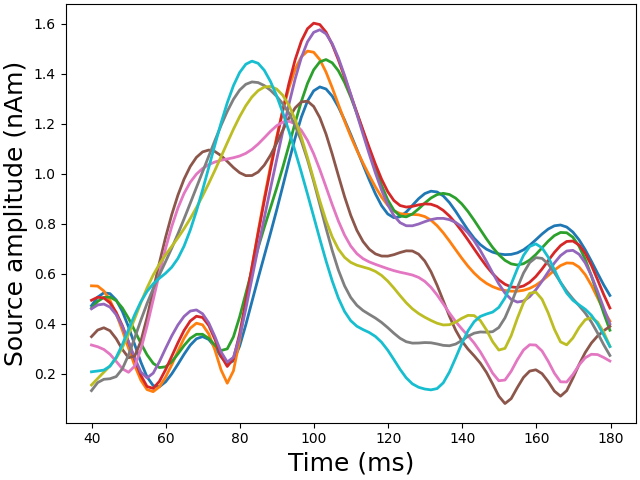
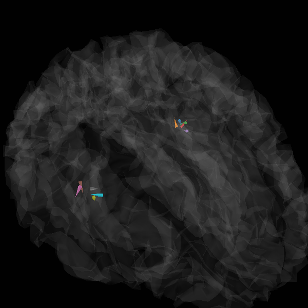
Total number of active sources: [ 56971 59453 61728 61772 68227 236975 240636 245391 250215 252407]
Total running time of the script: (0 minutes 3.702 seconds)