Regression-based baseline correction

This tutorial compares traditional baseline correction (adding or subtracting a scalar amount from every timepoint in an epoch) to a regression-based approach to baseline correction (which allows the effect of the baseline period to vary by timepoint). Specifically, this tutorial follows the method introduced by Alday[1].

There are at least two reasons you might consider using regression-based baseline correction:

1. Unlike traditional baseline correction, the regression-based approach does not assume that the effect of the baseline is equivalent between different experimental conditions. Thus it is safer against introduced bias.

2. Assuming that pre-trial baseline signal level is mostly determined by slow drifts in the data, the further away (in time) you get from the baseline period, the less likely it is that the signal level is similar in amplitude to the baseline amplitude. Thus using a time-varying baseline correction is less likely to introduce signal distortions / spurious effects in the later spans of long-duration epochs.

One issue that affects both traditional and regression-based baseline correction is the question of what time window to choose as the baseline window.

# Authors: Carina Forster
# Email: carinaforster0611@gmail.com

# License: BSD-3-Clause
# Copyright the MNE-Python contributors.

import numpy as np

import mne

Load the data

We’ll start by loading the MNE-Python sample dataset and extracting the experimental events to get trial locations and trial types. Since for this tutorial we’re only going to look at EEG channels, we can drop the other channel types, to speed things up:

data_path = mne.datasets.sample.data_path()
raw_fname = data_path / "MEG" / "sample" / "sample_audvis_filt-0-40_raw.fif"
raw = mne.io.read_raw_fif(raw_fname, preload=True)

events = mne.find_events(raw)

raw.pick(picks="eeg")

Opening raw data file /home/circleci/mne_data/MNE-sample-data/MEG/sample/sample_audvis_filt-0-40_raw.fif...
    Read a total of 4 projection items:
        PCA-v1 (1 x 102)  idle
        PCA-v2 (1 x 102)  idle
        PCA-v3 (1 x 102)  idle
        Average EEG reference (1 x 60)  idle
    Range : 6450 ... 48149 =     42.956 ...   320.665 secs
Ready.
Reading 0 ... 41699  =      0.000 ...   277.709 secs...
319 events found on stim channel STI 014
Event IDs: [ 1  2  3  4  5 32]

General

Measurement date	December 03, 2002 19:01:10 GMT
Experimenter	Unknown
Participant	Unknown

Channels

Digitized points	146 points
Good channels	59 EEG
Bad channels	EEG 053
EOG channels	Not available
ECG channels	Not available

Data

Sampling frequency	150.15 Hz
Highpass	0.10 Hz
Lowpass	40.00 Hz
Projections	Average EEG reference : off
Filenames	sample_audvis_filt-0-40_raw.fif
Duration	00:04:38 (HH:MM:SS)

Here we merge visual and auditory events from both hemispheres, and make our event_id dictionary for use during epoching.

events = mne.merge_events(events, [1, 2], 1)  # auditory events will be "1"
events = mne.merge_events(events, [3, 4], 2)  # visual events will be "2"
event_id = {"auditory": 1, "visual": 2}

Preprocessing

Next we’ll define some variables needed to epoch and preprocess the data. We’ll be combining left- and right-side stimuli, so we’ll look at a single central electrode to visualize the difference between auditory and visual trials.

tmin, tmax = -0.2, 0.5
lowpass, highpass = 40, 0.1
baseline_tmin, baseline_tmax = None, 0  # None takes the first timepoint
ch = "EEG 021"

We’ll do some standard preprocessing (a bandpass filter) and then epoch the data. Note that we don’t baseline correct the epochs (we specify baseline=None); we just minimally clean the data by rejecting channels with very high or low amplitudes. Note also that we operate on a copy of the data so that we can later compare this with traditional baselining.

raw_filtered = raw.copy().filter(highpass, lowpass)

epochs = mne.Epochs(
    raw_filtered,
    events,
    event_id,
    tmin=tmin,
    tmax=tmax,
    reject=dict(eeg=150e-6),
    flat=dict(eeg=5e-6),
    baseline=None,
    preload=True,
)

Filtering raw data in 1 contiguous segment
Setting up band-pass filter from 0.1 - 40 Hz

FIR filter parameters
---------------------
Designing a one-pass, zero-phase, non-causal bandpass filter:
- Windowed time-domain design (firwin) method
- Hamming window with 0.0194 passband ripple and 53 dB stopband attenuation
- Lower passband edge: 0.10
- Lower transition bandwidth: 0.10 Hz (-6 dB cutoff frequency: 0.05 Hz)
- Upper passband edge: 40.00 Hz
- Upper transition bandwidth: 10.00 Hz (-6 dB cutoff frequency: 45.00 Hz)
- Filter length: 4957 samples (33.013 s)

[Parallel(n_jobs=1)]: Done  17 tasks      | elapsed:    0.0s
Not setting metadata
288 matching events found
No baseline correction applied
Created an SSP operator (subspace dimension = 1)
1 projection items activated
Using data from preloaded Raw for 288 events and 106 original time points ...
    Rejecting  epoch based on EEG : ['EEG 001', 'EEG 002', 'EEG 003', 'EEG 007']
1 bad epochs dropped

Traditional baselining

First let’s baseline correct the data the traditional way. We average epochs within each condition, and subtract the condition-specific baseline separately for auditory and visual trials.

baseline = (baseline_tmin, baseline_tmax)
trad_aud = epochs["auditory"].average().apply_baseline(baseline)
trad_vis = epochs["visual"].average().apply_baseline(baseline)

Applying baseline correction (mode: mean)
Applying baseline correction (mode: mean)

Regression-based baselining

Now let’s try out the regression-based baseline correction approach. We’ll use mne.stats.linear_regression(), which needs a design matrix to represent the regression predictors. We’ll use four predictors: one for each experimental condition, one for the effect of baseline, and one that is an interaction between the baseline and one of the conditions (to account for any heterogeneity of the effect of baseline between the two conditions). Here are the first two:

aud_predictor = epochs.events[:, 2] == epochs.event_id["auditory"]
vis_predictor = epochs.events[:, 2] == epochs.event_id["visual"]

The baseline predictor is a bit trickier to compute: we’ll find the average value within the baseline period separately for each epoch, and use that value as our (trial-level) predictor. Here, since we’re focused on one particular channel, we’ll use the baseline value in that channel as our predictor, but depending on your research question you may want to do this seaprately for each channel or combine information across channels.

baseline_predictor = (
    epochs.copy()
    .crop(*baseline)
    .pick([ch])
    .get_data(copy=False)  # convert to NumPy array
    .mean(axis=-1)  # average across timepoints
    .squeeze()  # only 1 channel, so remove singleton dimension
)
baseline_predictor *= 1e6  # convert V → μV

Note that we converted just the predictor (not the epochs data) from Volts to microVolts. This is done for regression-model-fitting purposes (very small values can make model fitting unstable).

Now we can set up the design matrix, stacking the 1-D predictors as rows, then transposing with .T to make them columns. Combining them into one array() will also automatically convert the boolean aud_predictor and vis_predictor into ones and zeros:

design_matrix = np.vstack(
    [
        aud_predictor,
        vis_predictor,
        baseline_predictor,
        baseline_predictor * vis_predictor,
    ]
).T

Finally we fit the regression model:

reg_model = mne.stats.linear_regression(
    epochs, design_matrix, names=["auditory", "visual", "baseline", "baseline:visual"]
)

Fitting linear model to epochs, (6360 targets, 4 regressors)
Done

The function returns a dictionary of mne.stats.regression.lm objects, which are each a namedtuple() with the various estimated values stored as if it were an Evoked object. Let’s inspect it:

print(reg_model.keys())
print(f"model attributes: {reg_model['auditory']._fields}")
print("values are stored in Evoked objects:")
print(reg_model["auditory"].t_val)

dict_keys(['auditory', 'visual', 'baseline', 'baseline:visual'])
model attributes: ('beta', 'stderr', 't_val', 'p_val', 'mlog10_p_val')
values are stored in Evoked objects:
<Evoked | '' (average, N=1), -0.1998 – 0.49949 s, baseline off, 60 ch, ~3.0 MB>

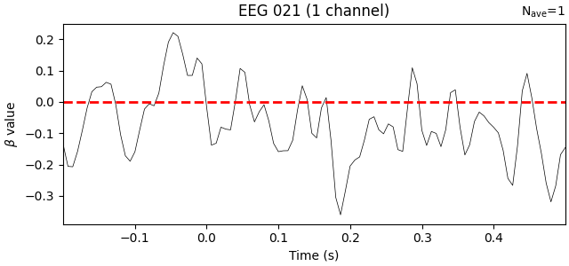
Plot the baseline regressor

First let’s look at the estimated effect of the baseline period. What we care about is the beta values, which tell us how strongly predictive the baseline value is at each timepoint. The model will estimate its effectiveness for every channel but since we used only one channel to form our baseline predictor, let’s examine how it looks for that channel only. We’ll add a horizontal line at β=1 to represent traditional baselining, where the effect is assumed to be constant across timepoints:

effect_of_baseline = reg_model["baseline"].beta
effect_of_baseline.plot(
    picks=ch,
    hline=[1.0],
    units=dict(eeg=r"$\beta$ value"),
    titles=dict(eeg=ch),
    selectable=False,
)

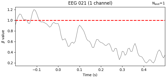
Unsurprisingly, the trend is that the farther away in time we get from the baseline period, the weaker the predictive value of the baseline amplitude becomes. Put another way, early time points (in this data) should be more strongly baseline-corrected than later time points.

Plot the ERPs

Now let’s look at the beta values for the two conditions (auditory and visual): these are the coefficients that represent the “pure” influence of the experimental stimuli on the signal, after taking into account the (time-varying!) effect of the baseline. We’ll plot them together, side-by-side with the traditional baseline approach:

reg_aud = reg_model["auditory"].beta
reg_vis = reg_model["visual"].beta

kwargs = dict(picks=ch, show_sensors=False, truncate_yaxis=False)
mne.viz.plot_compare_evokeds(
    dict(auditory=trad_aud, visual=trad_vis), title="Traditional", **kwargs
)
mne.viz.plot_compare_evokeds(
    dict(auditory=reg_aud, visual=reg_vis), title="Regression-based", **kwargs
)

• 
• 

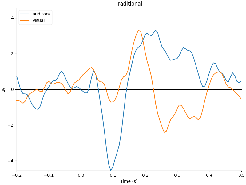
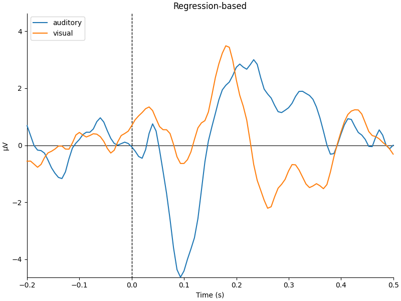
They look pretty similar, but there are some subtle differences in how far apart the two conditions are (e.g., around 400-500 ms).

Plot the scalp topographies and difference waves

Now let’s compare the scalp topographies for the traditional and regression-based approach. We’ll do this by computing the difference between conditions:

diff_traditional = mne.combine_evoked([trad_aud, trad_vis], weights=[1, -1])
diff_regression = mne.combine_evoked([reg_aud, reg_vis], weights=[1, -1])

Before we plot, let’s make sure we get the same color scale for both figures:

vmin = min(diff_traditional.get_data().min(), diff_regression.get_data().min()) * 1e6
vmax = max(diff_traditional.get_data().max(), diff_regression.get_data().max()) * 1e6
topo_kwargs = dict(vlim=(vmin, vmax), ch_type="eeg", times=np.linspace(0.05, 0.45, 9))

fig = diff_traditional.plot_topomap(**topo_kwargs)
fig.suptitle("Traditional")

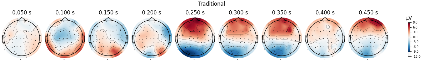
fig = diff_regression.plot_topomap(**topo_kwargs)
fig.suptitle("Regression-based")

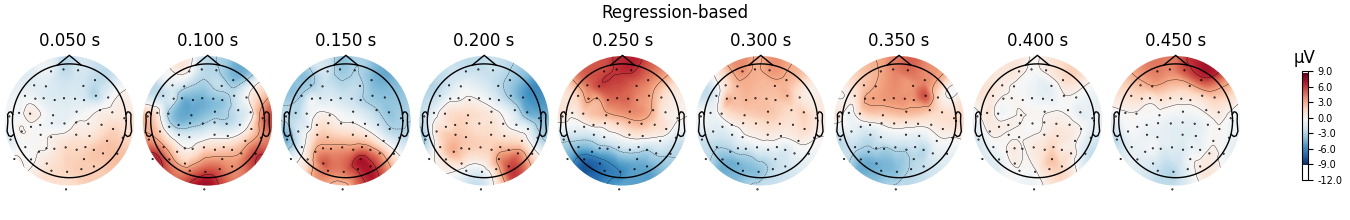
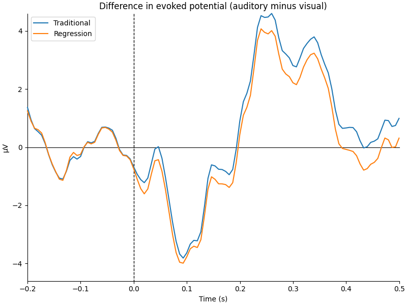
We can see that the regression-based approach shows stronger difference between conditions early on (around 100-150 ms) and weaker differences later (around 250-350 ms, and again around 450 ms). This is also reflected in the difference waves themselves: notice how the regression-based difference wave is further from zero around 150 ms but closer to zero around 250-350 ms.

title = "Difference in evoked potential (auditory minus visual)"
fig = mne.viz.plot_compare_evokeds(
    dict(Traditional=diff_traditional, Regression=diff_regression),
    title=title,
    **kwargs,
)

Examine the interaction term

Finally, let’s look at the interaction term from the regression model. This tells us whether the effect of the baseline period is different in the visual trials versus its effect in the auditory trials. Here we’ll add a horizontal line at zero, indicating the assumption that there ought to be no difference (i.e., baselines should not be systematically higher in one type of trial, and there should not be a difference in how long the effect of the baseline persists through time in each type of trial).

interaction_effect = reg_model["baseline:visual"].beta
interaction_effect.plot(
    picks=ch,
    hline=[0.0],
    units=dict(eeg=r"$\beta$ value"),
    titles=dict(eeg=ch),
    selectable=False,
)

Indeed, the interaction beta weights are rather small and seem to fluctuate randomly around zero, suggesting that there is no systematic difference in the effect of the baseline on our two trial types.

References

[1]

Phillip M. Alday. How much baseline correction do we need in ERP research? extended GLM model can replace baseline correction while lifting its limits. Psychophysiology, 2019. doi:10.1111/psyp.13451.

Estimated memory usage: 9 MB