Compute power and phase lock in label of the source space

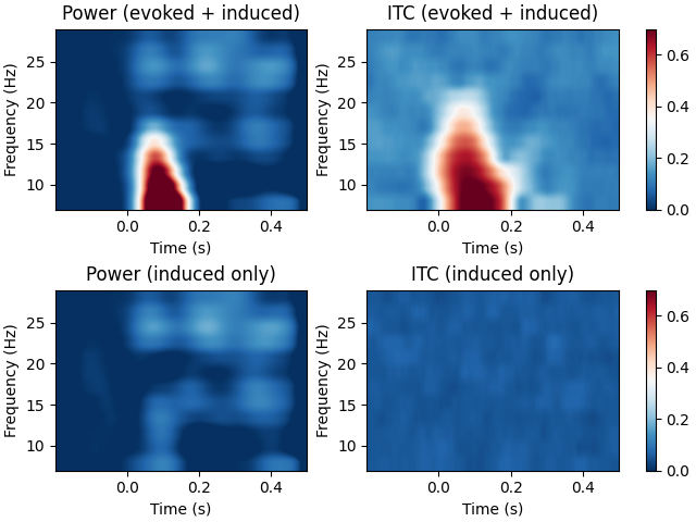
Compute time-frequency maps of power and phase lock in the source space. The inverse method is linear based on dSPM inverse operator.

The example also shows the difference in the time-frequency maps when they are computed with and without subtracting the evoked response from each epoch. The former results in induced activity only while the latter also includes evoked (stimulus-locked) activity.

# Authors: Alexandre Gramfort <alexandre.gramfort@inria.fr>
#
# License: BSD-3-Clause
# Copyright the MNE-Python contributors.

import matplotlib.pyplot as plt
import numpy as np

import mne
from mne import io
from mne.datasets import sample
from mne.minimum_norm import read_inverse_operator, source_induced_power

print(__doc__)

Set parameters

data_path = sample.data_path()
meg_path = data_path / "MEG" / "sample"
raw_fname = meg_path / "sample_audvis_raw.fif"
fname_inv = meg_path / "sample_audvis-meg-oct-6-meg-inv.fif"
label_names = ["Aud-lh", "Aud-rh"]
fname_labels = [meg_path / "labels" / f"{ln}.label" for ln in label_names]

tmin, tmax, event_id = -0.2, 0.5, 2

# Setup for reading the raw data
raw = io.read_raw_fif(raw_fname)
events = mne.find_events(raw, stim_channel="STI 014")
inverse_operator = read_inverse_operator(fname_inv)

include = []
raw.info["bads"] += ["MEG 2443", "EEG 053"]  # bads + 2 more

# Picks MEG channels
picks = mne.pick_types(
    raw.info, meg=True, eeg=False, eog=True, stim=False, include=include, exclude="bads"
)
reject = dict(grad=4000e-13, mag=4e-12, eog=150e-6)

# Load epochs
epochs = mne.Epochs(
    raw,
    events,
    event_id,
    tmin,
    tmax,
    picks=picks,
    baseline=(None, 0),
    reject=reject,
    preload=True,
)

# Compute a source estimate per frequency band including and excluding the
# evoked response
freqs = np.arange(7, 30, 2)  # define frequencies of interest
labels = [mne.read_label(fl) for fl in fname_labels]
label = labels[0]
n_cycles = freqs / 3.0  # different number of cycle per frequency

# subtract the evoked response in order to exclude evoked activity
epochs_induced = epochs.copy().subtract_evoked()

fig, axes = plt.subplots(2, 2, layout="constrained")
for ii, (this_epochs, title) in enumerate(
    zip([epochs, epochs_induced], ["evoked + induced", "induced only"])
):
    # compute the source space power and the inter-trial coherence
    power, itc = source_induced_power(
        this_epochs,
        inverse_operator,
        freqs,
        label,
        baseline=(-0.1, 0),
        baseline_mode="percent",
        n_cycles=n_cycles,
        n_jobs=None,
    )

    power = np.mean(power, axis=0)  # average over sources
    itc = np.mean(itc, axis=0)  # average over sources
    times = epochs.times

    ##########################################################################
    # View time-frequency plots
    ax = axes[ii, 0]
    ax.imshow(
        20 * power,
        extent=[times[0], times[-1], freqs[0], freqs[-1]],
        aspect="auto",
        origin="lower",
        vmin=0.0,
        vmax=30.0,
        cmap="RdBu_r",
    )
    ax.set(xlabel="Time (s)", ylabel="Frequency (Hz)", title=f"Power ({title})")

    ax = axes[ii, 1]
    ax.imshow(
        itc,
        extent=[times[0], times[-1], freqs[0], freqs[-1]],
        aspect="auto",
        origin="lower",
        vmin=0,
        vmax=0.7,
        cmap="RdBu_r",
    )
    ax.set(xlabel="Time (s)", ylabel="Frequency (Hz)", title=f"ITC ({title})")
    fig.colorbar(ax.images[0], ax=axes[ii])

Opening raw data file /home/circleci/mne_data/MNE-sample-data/MEG/sample/sample_audvis_raw.fif...
    Read a total of 3 projection items:
        PCA-v1 (1 x 102)  idle
        PCA-v2 (1 x 102)  idle
        PCA-v3 (1 x 102)  idle
    Range : 25800 ... 192599 =     42.956 ...   320.670 secs
Ready.
Finding events on: STI 014
320 events found on stim channel STI 014
Event IDs: [ 1  2  3  4  5 32]
Reading inverse operator decomposition from /home/circleci/mne_data/MNE-sample-data/MEG/sample/sample_audvis-meg-oct-6-meg-inv.fif...
    Reading inverse operator info...
    [done]
    Reading inverse operator decomposition...
    [done]
    305 x 305 full covariance (kind = 1) found.
    Read a total of 4 projection items:
        PCA-v1 (1 x 102) active
        PCA-v2 (1 x 102) active
        PCA-v3 (1 x 102) active
        Average EEG reference (1 x 60) active
    Noise covariance matrix read.
    22494 x 22494 diagonal covariance (kind = 2) found.
    Source covariance matrix read.
    22494 x 22494 diagonal covariance (kind = 6) found.
    Orientation priors read.
    22494 x 22494 diagonal covariance (kind = 5) found.
    Depth priors read.
    Did not find the desired covariance matrix (kind = 3)
    Reading a source space...
    Computing patch statistics...
    Patch information added...
    Distance information added...
    [done]
    Reading a source space...
    Computing patch statistics...
    Patch information added...
    Distance information added...
    [done]
    2 source spaces read
    Read a total of 4 projection items:
        PCA-v1 (1 x 102) active
        PCA-v2 (1 x 102) active
        PCA-v3 (1 x 102) active
        Average EEG reference (1 x 60) active
    Source spaces transformed to the inverse solution coordinate frame
Not setting metadata
73 matching events found
Setting baseline interval to [-0.19979521315838786, 0.0] s
Applying baseline correction (mode: mean)
Created an SSP operator (subspace dimension = 3)
3 projection items activated
Loading data for 73 events and 421 original time points ...
    Rejecting  epoch based on EOG : ['EOG 061']
    Rejecting  epoch based on EOG : ['EOG 061']
    Rejecting  epoch based on EOG : ['EOG 061']
    Rejecting  epoch based on EOG : ['EOG 061']
    Rejecting  epoch based on EOG : ['EOG 061']
    Rejecting  epoch based on MAG : ['MEG 1711']
    Rejecting  epoch based on EOG : ['EOG 061']
    Rejecting  epoch based on EOG : ['EOG 061']
    Rejecting  epoch based on EOG : ['EOG 061']
    Rejecting  epoch based on EOG : ['EOG 061']
    Rejecting  epoch based on EOG : ['EOG 061']
    Rejecting  epoch based on EOG : ['EOG 061']
    Rejecting  epoch based on EOG : ['EOG 061']
    Rejecting  epoch based on EOG : ['EOG 061']
14 bad epochs dropped
Subtracting Evoked from Epochs
    The following channels are not included in the subtraction: EOG 061
[done]
Preparing the inverse operator for use...
    Scaled noise and source covariance from nave = 1 to nave = 1
    Created the regularized inverter
    Created an SSP operator (subspace dimension = 3)
    Created the whitener using a noise covariance matrix with rank 302 (3 small eigenvalues omitted)
    Computing noise-normalization factors (dSPM)...
[done]
Picked 305 channels from the data
Computing inverse...
    Eigenleads need to be weighted ...
Reducing data rank 99 -> 99
Computing source power ...
Outputting power for 33 vertices in label Aud-lh.
Applying baseline correction (mode: percent)
Preparing the inverse operator for use...
    Scaled noise and source covariance from nave = 1 to nave = 1
    Created the regularized inverter
    Created an SSP operator (subspace dimension = 3)
    Created the whitener using a noise covariance matrix with rank 302 (3 small eigenvalues omitted)
    Computing noise-normalization factors (dSPM)...
[done]
Picked 305 channels from the data
Computing inverse...
    Eigenleads need to be weighted ...
Reducing data rank 99 -> 99
Computing source power ...
Outputting power for 33 vertices in label Aud-lh.
Applying baseline correction (mode: percent)

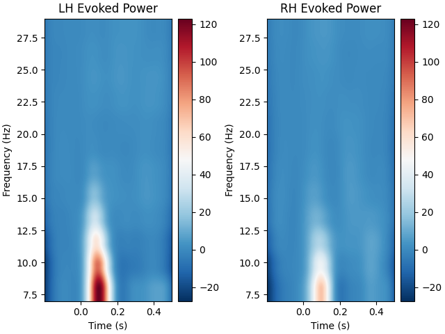
In the example above, we averaged power across vertices after calculating power because we provided a single label for power calculation and therefore power of all sources within the single label were returned separately. When we provide a list of labels, power is averaged across sources within each label automatically. With a list of labels, averaging is performed before rescaling, so choose a baseline method appropriately.

# Get power from multiple labels
multi_label_power = source_induced_power(
    epochs,
    inverse_operator,
    freqs,
    labels,
    baseline=(-0.1, 0),
    baseline_mode="mean",
    n_cycles=n_cycles,
    n_jobs=None,
    return_plv=False,
)

# visually compare evoked power in left and right auditory regions
fig, axes = plt.subplots(ncols=2, layout="constrained")
for l_idx, l_power in enumerate(multi_label_power):
    ax = axes[l_idx]
    ax.imshow(
        l_power,
        extent=[epochs.times[0], epochs.times[-1], freqs[0], freqs[-1]],
        aspect="auto",
        origin="lower",
        vmin=multi_label_power.min(),
        vmax=multi_label_power.max(),
        cmap="RdBu_r",
    )
    title = f"{labels[l_idx].hemi.upper()} Evoked Power"
    ax.set(xlabel="Time (s)", ylabel="Frequency (Hz)", title=title)
    fig.colorbar(ax.images[0], ax=ax)

Preparing the inverse operator for use...
    Scaled noise and source covariance from nave = 1 to nave = 1
    Created the regularized inverter
    Created an SSP operator (subspace dimension = 3)
    Created the whitener using a noise covariance matrix with rank 302 (3 small eigenvalues omitted)
    Computing noise-normalization factors (dSPM)...
[done]
Picked 305 channels from the data
Computing inverse...
    Eigenleads need to be weighted ...
Reducing data rank 180 -> 180
Computing source power ...
Averaging induced power across vertices within labels for 2 labels.
Applying baseline correction (mode: mean)