Note
Go to the end to download the full example code.
Working with sensor locations#
This tutorial describes how to read and plot sensor locations, and how MNE-Python handles physical locations of sensors. As usual we’ll start by importing the modules we need:
# Authors: The MNE-Python contributors.
# License: BSD-3-Clause
# Copyright the MNE-Python contributors.
from pathlib import Path

import matplotlib.pyplot as plt
import numpy as np

import mne
About montages and layouts#
Montages contain sensor positions in 3D (x, y, z in
meters), which can be assigned to existing EEG/MEG data. By specifying the locations
of sensors relative to the brain, Montages play an
important role in computing the forward solution and inverse estimates.
In contrast, Layouts are idealized 2D representations of
sensor positions. They are primarily used for arranging individual sensor subplots in
a topoplot or for showing the approximate relative arrangement of sensors as seen
from above.
Note
If you’re working with EEG data exclusively, you’ll want to use Montages, not layouts. Idealized montages (e.g., those provided
by the manufacturer, or the ones shipping with MNE-Python mentioned below) are
typically referred to as template montages.
Working with built-in montages#
The 3D coordinates of MEG sensors are included in the raw recordings from MEG systems.
They are automatically stored in the info attribute of the Raw object
upon loading. EEG electrode locations are much more variable because of differences in
head shape. Idealized montages (”template montages”) for
many EEG systems are included in MNE-Python, and you can get an overview of them by
using mne.channels.get_builtin_montages():
builtin_montages = mne.channels.get_builtin_montages(descriptions=True)
for montage_name, montage_description in builtin_montages:
    print(f"{montage_name}: {montage_description}")
fsaverage_1005: Electrodes are named according to the international 10-05 system and positioned on the fsaverage head model (335+3 locations)
fsaverage_1010: Electrodes are named according to the international 10-10 system and positioned on the fsaverage head model (70+3 locations)
fsaverage_1020: Electrodes are named according to the international 10-20 system and positioned on the fsaverage head model (21+3 locations)
colin27_1005: Electrodes are named according to the international 10-05 system and positioned on the Colin27 head model (343+3 locations)
colin27_1020: Electrodes are named according to the international extended 10-20 system and positioned on the Colin27 head model (94+3 locations)
colin27_alphabetic: Electrodes are named with LETTER-NUMBER combinations (A1, B2, F4, …) and positioned on the Colin27 head model (65+3 locations)
colin27_postfixed: Electrodes are named according to the international extended 10-20 system using postfixes for intermediate positions and positioned on the Colin27 head model (100+3 locations)
colin27_prefixed: Electrodes are named according to the international extended 10-20 system using prefixes for intermediate positions and positioned on the Colin27 head model (74+3 locations)
colin27_primed: Electrodes are named according to the international extended 10-20 system using prime marks (' and '') for intermediate positions and positioned on the Colin27 head model (100+3 locations)
biosemi16: BioSemi cap with 16 electrodes (16+3 locations)
biosemi32: BioSemi cap with 32 electrodes (32+3 locations)
biosemi64: BioSemi cap with 64 electrodes (64+3 locations)
biosemi128: BioSemi cap with 128 electrodes (128+3 locations)
biosemi160: BioSemi cap with 160 electrodes (160+3 locations)
biosemi256: BioSemi cap with 256 electrodes (256+3 locations)
easycap-M1: EasyCap with 10-05 electrode names (74+3 locations)
easycap-M10: EasyCap with numbered electrodes (61+3 locations)
easycap-M43: EasyCap with numbered electrodes (64+3 locations)
EGI_256: Geodesic Sensor Net (256+3 locations)
GSN-HydroCel-32: HydroCel Geodesic Sensor Net and Cz (33+3 locations)
GSN-HydroCel-64_1.0: HydroCel Geodesic Sensor Net (64+3 locations)
GSN-HydroCel-65_1.0: HydroCel Geodesic Sensor Net and Cz (65+3 locations)
GSN-HydroCel-128: HydroCel Geodesic Sensor Net (128+3 locations)
GSN-HydroCel-129: HydroCel Geodesic Sensor Net and Cz (129+3 locations)
GSN-HydroCel-256: HydroCel Geodesic Sensor Net (256+3 locations)
GSN-HydroCel-257: HydroCel Geodesic Sensor Net and Cz (257+3 locations)
mgh60: The (older) 60-channel cap used at MGH (60+3 locations)
mgh70: The (newer) 70-channel BrainVision cap used at MGH (70+3 locations)
artinis-octamon: Artinis OctaMon fNIRS (8 sources, 2 detectors)
artinis-brite23: Artinis Brite23 fNIRS (11 sources, 7 detectors)
brainproducts-RNP-BA-128: Brain Products with 10-10 electrode names (130+3 locations)
spherical_1005: 10–05 electrode names and locations using a spherical head model (344+3 locations)
spherical_1010: 10–10 electrode names and locations using a spherical head model (70+3 locations)
spherical_1020: 10–20 electrode names and locations using a spherical head model (21+3 locations)
These built-in EEG montages can be loaded with mne.channels.make_standard_montage:
easycap_montage = mne.channels.make_standard_montage("easycap-M1")
print(easycap_montage)
<DigMontage | 0 extras (headshape), 0 HPIs, 3 fiducials, 74 channels>
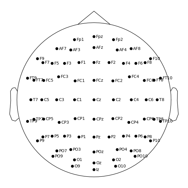
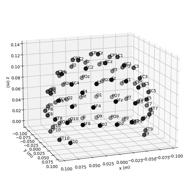
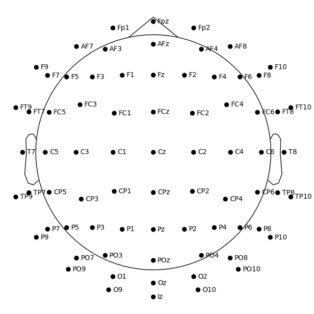
Montage objects have a plot
method for visualizing the sensor locations in 2D or 3D:
easycap_montage.plot()  # 2D
fig = easycap_montage.plot(kind="3d", show=False)  # 3D
fig = fig.gca().view_init(azim=70, elev=15)  # set view angle for tutorial
Once loaded, a montage can be applied to data with the set_montage
method, for example raw.set_montage(),
epochs.set_montage(), or evoked.set_montage(). This will only work with data whose EEG channel names
correspond to those in the montage. (Therefore, we’re loading some EEG data below, and
not the usual MNE “sample” dataset.)
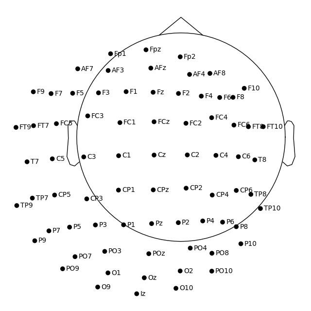
You can then visualize the sensor locations via the plot_sensors()
method.
It is also possible to skip the manual montage loading step by passing the montage
name directly to the set_montage() method.
ssvep_folder = mne.datasets.ssvep.data_path()
ssvep_data_raw_path = (
    ssvep_folder / "sub-02" / "ses-01" / "eeg" / "sub-02_ses-01_task-ssvep_eeg.vhdr"
)
ssvep_raw = mne.io.read_raw_brainvision(ssvep_data_raw_path, verbose=False)

# Use the preloaded montage
ssvep_raw.set_montage(easycap_montage)
fig = ssvep_raw.plot_sensors(show_names=True)

# Apply a template montage directly, without preloading
ssvep_raw.set_montage("easycap-M1")
fig = ssvep_raw.plot_sensors(show_names=True)

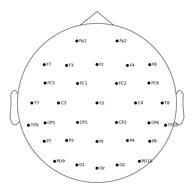
Note
You may have noticed that the figures created via plot_sensors()
contain fewer sensors than the result of easycap_montage.plot(). This is because the montage contains all channels
defined for that EEG system; but not all recordings will necessarily use all
possible channels. Thus when applying a montage to an actual EEG dataset,
information about sensors that are not actually present in the data is removed.
Plotting 2D sensor locations like EEGLAB#
In MNE-Python, by default the head center is calculated using fiducial points. This means that the head circle represents the head circumference at the nasion and ear level, and not where it is commonly measured in the 10–20 EEG system (i.e., above the nasion at T4/T8, T3/T7, Oz, and Fpz).
If you prefer to draw the head circle using 10–20 conventions (which are also used by
EEGLAB), you can pass sphere='eeglab':
fig = ssvep_raw.plot_sensors(show_names=True, sphere="eeglab")
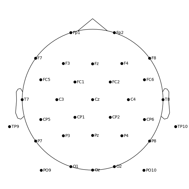
Approximating Fpz location by mirroring Oz along the X and Y axes.
Because the data we’re using here doesn’t contain an Fpz channel, its putative location was approximated automatically.
Manually controlling 2D channel projection#
Channel positions in 2D space are obtained by projecting their actual 3D positions
onto a sphere, then projecting the sphere onto a plane. By default, a sphere with
origin at (0, 0, 0) (x, y, z coordinates) and radius of 0.095 meters (9.5 cm)
is used. You can use a different sphere radius by passing a single value as the
sphere argument in any function that plots channels in 2D (like
plot that we use here, but also for example
mne.viz.plot_topomap):
fig1 = easycap_montage.plot()  # default radius of 0.095
fig2 = easycap_montage.plot(sphere=0.07)

To change not only the radius, but also the sphere origin, pass a
(x, y, z, radius) tuple as the sphere argument:
fig = easycap_montage.plot(sphere=(0.03, 0.02, 0.01, 0.075))
Reading sensor digitization files#
In the sample data, the sensor positions are already available in the info
attribute of the Raw object (see the documentation of the reading functions
and set_montage() for details on how that works). Therefore, we can
plot sensor locations directly from the Raw object using
plot_sensors(), which provides similar functionality to
montage.plot(). In addition,
plot_sensors() supports channel selection by type, color-coding
channels in various ways (by default, channels listed in raw.info['bads'] will be
plotted in red), and drawing in an existing Matplotlib Axes object (so the channel
positions can easily be added as a subplot in a multi-panel figure):
sample_data_folder = mne.datasets.sample.data_path()
sample_data_raw_path = sample_data_folder / "MEG" / "sample" / "sample_audvis_raw.fif"
sample_raw = mne.io.read_raw_fif(sample_data_raw_path, preload=False, verbose=False)

fig = plt.figure()
ax2d = fig.add_subplot(121)
ax3d = fig.add_subplot(122, projection="3d")
sample_raw.plot_sensors(ch_type="eeg", axes=ax2d)
sample_raw.plot_sensors(ch_type="eeg", axes=ax3d, kind="3d")
ax3d.view_init(azim=70, elev=15)
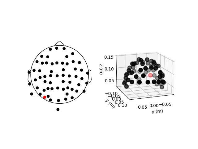
The previous 2D topomap reveals irregularities in the EEG sensor positions in the
sample dataset — this is because the sensor positions in that
dataset are digitizations of actual sensor positions on the head rather than idealized
sensor positions based on a spherical head model. Depending on the digitization device
(e.g., a Polhemus Fastrak digitizer), you need to use different montage reading
functions (see Supported formats for digitized 3D locations). The resulting montage
can then be added to Raw objects by passing it as an argument to the
set_montage() method (just as we did before with the name of the
predefined 'spherical_1020' montage). Once loaded, locations can be plotted with
the plot() method and saved with the
save() method of the
montage object.
Note
When setting a montage with set_montage(), the measurement info
is updated in two places (both chs and dig entries are updated) – see
The Info data structure for more details. Note that dig may contain HPI,
fiducial, or head shape points in addition to electrode locations.
Visualizing sensors in 3D surface renderings#
It is also possible to render an image of an MEG sensor helmet using 3D surface
rendering instead of matplotlib. This works by calling mne.viz.plot_alignment():
fig = mne.viz.plot_alignment(
    sample_raw.info,
    dig=False,
    eeg=False,
    surfaces=[],
    meg=["helmet", "sensors"],
    coord_frame="meg",
)
mne.viz.set_3d_view(fig, azimuth=50, elevation=90, distance=0.5)
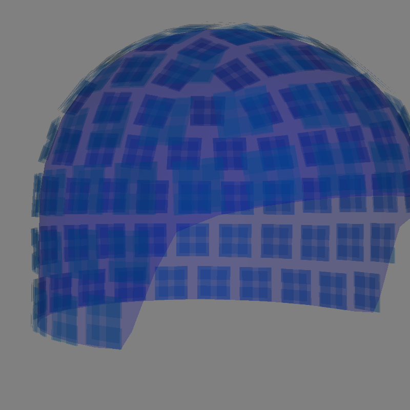
Getting helmet for system 306m
Channel types:: grad: 203, mag: 102
Note that plot_alignment() requires an Info object, and can also
render MRI surfaces of the scalp, skull, and brain (by passing a dict with keys like
'head', 'outer_skull' or 'brain' to the surfaces parameter). This
makes the function useful for assessing coordinate frame transformations. For examples of various uses of
plot_alignment(), see Plotting sensor layouts of EEG systems, Plotting EEG sensors on the scalp, and
Plotting sensor layouts of MEG systems.
Working with layout files#
Similar to montages, many layout files are included with MNE-Python. They are stored
in the mne/channels/data/layouts folder:
layout_dir = Path(mne.__file__).parent / "channels" / "data" / "layouts"
layouts = sorted(path.name for path in layout_dir.iterdir())
print("\nBUILT-IN LAYOUTS\n================")
print("\n".join(layouts))
BUILT-IN LAYOUTS
================
CTF-275.lout
CTF151.lay
CTF275.lay
EEG1005.lay
EGI256.lout
GeodesicHeadWeb-130.lout
GeodesicHeadWeb-280.lout
KIT-125.lout
KIT-157.lout
KIT-160.lay
KIT-AD.lout
KIT-AS-2008.lout
KIT-UMD-3.lout
Neuromag_122.lout
Vectorview-all.lout
Vectorview-grad.lout
Vectorview-grad_norm.lout
Vectorview-mag.lout
biosemi.lay
magnesWH3600.lout
To load a layout file, use the mne.channels.read_layout function. You can then
visualize the layout using its plot method:
biosemi_layout = mne.channels.read_layout("biosemi")
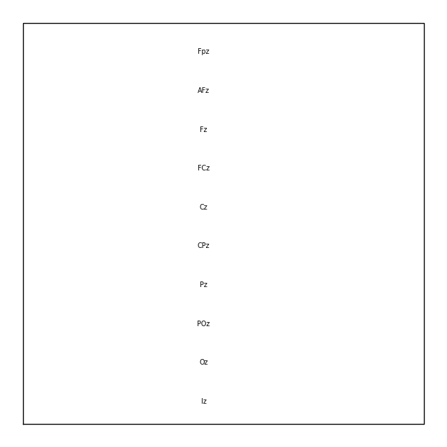
Similar to the picks argument for selecting channels from Raw objects,
the plot() method of Layout objects also
has a picks argument. However, because layouts only contain information about
sensor name and location (not sensor type), the plot()
method only supports picking channels by index (not by name or by type). In the
following example, we find the desired indices using numpy.where(); selection by
name or type is possible with mne.pick_channels() or mne.pick_types().
midline = np.where([name.endswith("z") for name in biosemi_layout.names])[0]
biosemi_layout.plot(picks=midline)
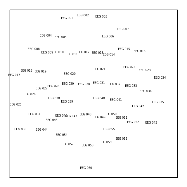
If you have a Raw object that contains sensor positions, you can create a
Layout object with either mne.channels.make_eeg_layout() or
mne.channels.find_layout().
layout_from_raw = mne.channels.make_eeg_layout(sample_raw.info)
# same result as mne.channels.find_layout(raw.info, ch_type='eeg')
layout_from_raw.plot()
Note
There is no corresponding make_meg_layout() function because sensor locations
are fixed in an MEG system (unlike in EEG, where sensor caps deform to fit snugly
on a specific head). Therefore, MEG layouts are consistent (constant) for a given
system and you can simply load them with mne.channels.read_layout() or use
mne.channels.find_layout() with the ch_type parameter (as previously
demonstrated for EEG).
All Layout objects have a save method that
writes layouts to disk as either .lout or .lay formats (inferred from
the file extension contained in the fname argument). The choice between
.lout and .lay format only matters if you need to load the layout file
in some other application (MNE-Python can read both formats).
Total running time of the script: (0 minutes 10.087 seconds)