Note
Go to the end to download the full example code.
The Raw data structure: continuous data#
This tutorial covers the basics of working with raw EEG/MEG data in Python. It
introduces the Raw data structure in detail, including how to
load, query, subselect, export, and plot data from a Raw
object. For more info on visualization of Raw objects, see
Built-in plotting methods for Raw objects. For info on creating a Raw object
from simulated data in a NumPy array, see
Creating MNE-Python data structures from scratch.
As usual we’ll start by importing the modules we need:
# Authors: The MNE-Python contributors.
# License: BSD-3-Clause
# Copyright the MNE-Python contributors.
import os

import matplotlib.pyplot as plt
import numpy as np

import mne
Loading continuous data#
As mentioned in the introductory tutorial,
MNE-Python data structures are based around
the .fif file format from Neuromag. This tutorial uses an
example dataset in .fif format, so here we’ll
use the function mne.io.read_raw_fif() to load the raw data; there are
reader functions for a wide variety of other data formats as well.
There are also several other example datasets that can be downloaded with just a few lines
of code. Functions for downloading example datasets are in the
mne.datasets submodule; here we’ll use
mne.datasets.sample.data_path() to download the “Sample”
dataset, which contains EEG, MEG, and structural MRI data from one subject
performing an audiovisual experiment. When it’s done downloading,
data_path() will return the folder location where
it put the files; you can navigate there with your file browser if you want
to examine the files yourself. Once we have the file path, we can load the
data with read_raw_fif(). This will return a
Raw object, which we’ll store in a variable called raw.
sample_data_folder = mne.datasets.sample.data_path()
sample_data_raw_file = os.path.join(
    sample_data_folder, "MEG", "sample", "sample_audvis_raw.fif"
)
raw = mne.io.read_raw_fif(sample_data_raw_file)
Opening raw data file /home/circleci/mne_data/MNE-sample-data/MEG/sample/sample_audvis_raw.fif...
    Read a total of 3 projection items:
        PCA-v1 (1 x 10²)  idle
        PCA-v2 (1 x 10²)  idle
        PCA-v3 (1 x 10²)  idle
    Range : 25800 ... 192599 =     42.956 ...   320.670 secs
Ready.
As you can see above, read_raw_fif() automatically displays
some information about the file it’s loading. For example, here it tells us
that there are three “projection items” in the file along with the recorded
data; those are SSP projectors calculated to remove
environmental noise from the MEG signals, and are discussed in a the tutorial
Background on projectors and projections.
In addition to the information displayed during loading, you can
get a glimpse of the basic details of a Raw object by
printing it:
print(raw)
<Raw | sample_audvis_raw.fif, 376 x 166800 (277.7 s), ~3.2 MiB, data not loaded>
By default, the mne.io.read_raw_* family of functions will not
load the data into memory (instead the data on disk are memory-mapped,
meaning the data are only read from disk as-needed). Some operations (such as
filtering) require that the data be copied into RAM; to do that we could have
passed the preload=True parameter to read_raw_fif(), but we
can also copy the data into RAM at any time using the
load_data() method. However, since this particular tutorial
doesn’t do any serious analysis of the data, we’ll first
crop() the Raw object to 60 seconds so it
uses less memory and runs more smoothly on our documentation server.
raw.crop(tmax=60)
Querying the Raw object#
We saw above that printing the Raw object displays some
basic information like the total number of channels, the number of time
points at which the data were sampled, total duration, and the approximate
size in memory. Much more information is available through the various
attributes and methods of the Raw class. Some useful
attributes of Raw objects include a list of the channel
names (ch_names), an array of the sample times in seconds
(times), and the total number of samples
(n_times); a list of all attributes and methods is given
in the documentation of the Raw class.
The Raw.info attribute#
There is also quite a lot of information stored in the raw.info
attribute, which stores an Info object that is similar to a
Python dictionary (in that it has fields accessed via named
keys). Like Python dictionaries, raw.info has a .keys() method that
shows all the available field names; unlike Python dictionaries, printing
raw.info will print a nicely-formatted glimpse of each field’s data. See
The Info data structure for more on what is stored in Info
objects, and how to interact with them.
n_time_samps = raw.n_times
time_secs = raw.times
ch_names = raw.ch_names
n_chan = len(ch_names)  # note: there is no raw.n_channels attribute
print(
    f"the (cropped) sample data object has {n_time_samps} time samples and "
    f"{n_chan} channels."
)
print(f"The last time sample is at {time_secs[-1]} seconds.")
print("The first few channel names are {}.".format(", ".join(ch_names[:3])))
print()  # insert a blank line in the output

# some examples of raw.info:
print("bad channels:", raw.info["bads"])  # chs marked "bad" during acquisition
print(raw.info["sfreq"], "Hz")  # sampling frequency
print(raw.info["description"], "\n")  # miscellaneous acquisition info

print(raw.info)
the (cropped) sample data object has 36038 time samples and 376 channels.
The last time sample is at 60.000167471573526 seconds.
The first few channel names are MEG 0113, MEG 0112, MEG 0111.

bad channels: ['MEG 2443', 'EEG 053']
600.614990234375 Hz
acquisition (megacq) VectorView system at NMR-MGH

<Info | 21 non-empty values
 acq_pars: ACQch001 110113 ACQch002 110112 ACQch003 110111 ACQch004 110122 ...
 bads: 2 items (MEG 2443, EEG 053)
 ch_names: MEG 0113, MEG 0112, MEG 0111, MEG 0122, MEG 0123, MEG 0121, MEG ...
 chs: 204 Gradiometers, 102 Magnetometers, 9 Stimulus, 60 EEG, 1 EOG
 custom_ref_applied: False
 description: acquisition (megacq) VectorView system at NMR-MGH
 dev_head_t: MEG device -> head transform
 dig: 146 items (3 Cardinal, 4 HPI, 61 EEG, 78 Extra)
 events: 1 item (list)
 experimenter: MEG
 file_id: 4 items (dict)
 highpass: 0.1 Hz
 hpi_meas: 1 item (list)
 hpi_results: 1 item (list)
 lowpass: 172.2 Hz
 meas_date: 2002-12-03 19:01:10 UTC
 meas_id: 4 items (dict)
 nchan: 376
 proj_id: 1
 proj_name: test
 projs: PCA-v1: off, PCA-v2: off, PCA-v3: off
 sfreq: 600.6 Hz
>
Note
Most of the fields of raw.info reflect metadata recorded at
acquisition time, and should not be changed by the user. There are a few
exceptions (such as raw.info['bads'] and raw.info['projs']), but
in most cases there are dedicated MNE-Python functions or methods to
update the Info object safely (such as
add_proj() to update raw.info['projs']).
Time, sample number, and sample index#
One method of Raw objects that is frequently useful is
time_as_index(), which converts a time (in seconds) into
the integer index of the sample occurring closest to that time. The method
can also take a list or array of times, and will return an array of indices.
It is important to remember that there may not be a data sample at exactly
the time requested, so the number of samples between time = 1 second and
time = 2 seconds may be different than the number of samples between
time = 2 and time = 3:
print(raw.time_as_index(20))
print(raw.time_as_index([20, 30, 40]), "\n")

print(np.diff(raw.time_as_index([1, 2, 3])))
[12012]
[12012 18018 24024]

[601 600]
Modifying Raw objects#
Raw objects have a number of methods that modify the
Raw instance in-place and return a reference to the modified
instance. This can be useful for method chaining
(e.g., raw.crop(...).pick(...).filter(...).plot())
but it also poses a problem during interactive analysis: if you modify your
Raw object for an exploratory plot or analysis (say, by
dropping some channels), you will then need to re-load the data (and repeat
any earlier processing steps) to undo the channel-dropping and try something
else. For that reason, the examples in this section frequently use the
copy() method before the other methods being demonstrated,
so that the original Raw object is still available in the
variable raw for use in later examples.
Selecting, dropping, and reordering channels#
Altering the channels of a Raw object can be done in several
ways. As a first example, we’ll use the pick() method
to restrict the Raw object to just the EEG and EOG channels:
eeg_and_eog = raw.copy().pick(picks=["eeg", "eog"])
print(len(raw.ch_names), "→", len(eeg_and_eog.ch_names))
376 → 61
In addition, pick() can also be used to pick channels by name, and a
corresponding drop_channels() method to remove channels by
name:
raw_temp = raw.copy()
print("Number of channels in raw_temp:")
print(len(raw_temp.ch_names), end=" → drop two → ")
raw_temp.drop_channels(["EEG 037", "EEG 059"])
print(len(raw_temp.ch_names), end=" → pick three → ")
raw_temp.pick(["MEG 1811", "EEG 017", "EOG 061"])
print(len(raw_temp.ch_names))
Number of channels in raw_temp:
376 → drop two → 374 → pick three → 3
If you want the channels in a specific order (e.g., for plotting),
reorder_channels() works just like
pick() but also reorders the channels; for
example, here we pick the EOG and frontal EEG channels, putting the EOG
first and the EEG in reverse order:
channel_names = ["EOG 061", "EEG 003", "EEG 002", "EEG 001"]
eog_and_frontal_eeg = raw.copy().reorder_channels(channel_names)
print(eog_and_frontal_eeg.ch_names)
['EOG 061', 'EEG 003', 'EEG 002', 'EEG 001']
Changing channel name and type#
You may have noticed that the EEG channel names in the sample data are
numbered rather than labelled according to a standard nomenclature such as
the 10-20 or 10-05 systems, or perhaps it
bothers you that the channel names contain spaces. It is possible to rename
channels using the rename_channels() method, which takes a
Python dictionary to map old names to new names. You need not rename all
channels at once; provide only the dictionary entries for the channels you
want to rename. Here’s a frivolous example:
raw.rename_channels({"EOG 061": "blink detector"})
This next example replaces spaces in the channel names with underscores, using a Python dict comprehension:
print(raw.ch_names[-3:])
channel_renaming_dict = {name: name.replace(" ", "_") for name in raw.ch_names}
raw.rename_channels(channel_renaming_dict)
print(raw.ch_names[-3:])
['EEG 059', 'EEG 060', 'blink detector']
['EEG_059', 'EEG_060', 'blink_detector']
If for some reason the channel types in your Raw object are
inaccurate, you can change the type of any channel with the
set_channel_types() method. The method takes a
dictionary mapping channel names to types; allowed types are
bio, chpi, csd, dbs, dipole, ecg, ecog, eeg, emg, eog, exci, eyegaze,
fnirs_cw_amplitude, fnirs_fd_ac_amplitude, fnirs_fd_phase, fnirs_od, gof,
gsr, hbo, hbr, ias, misc, pupil, ref_meg, resp, seeg, stim, syst,
temperature
(see sensor types for more information about them).
A common use case for changing channel type is when using frontal EEG
electrodes as makeshift EOG channels:
raw.set_channel_types({"EEG_001": "eog"})
print(raw.copy().pick(picks="eog").ch_names)
['EEG_001', 'blink_detector']
Selection in the time domain#
If you want to limit the time domain of a Raw object, you
can use the crop() method, which modifies the
Raw object in place (we’ve seen this already at the start of
this tutorial, when we cropped the Raw object to 60 seconds
to reduce memory demands). crop() takes parameters tmin
and tmax, both in seconds (here we’ll again use copy()
first to avoid changing the original Raw object):
raw_selection = raw.copy().crop(tmin=10, tmax=12.5)
print(raw_selection)
<Raw | sample_audvis_raw.fif, 376 x 1503 (2.5 s), ~3.2 MiB, data not loaded>
crop() also modifies the first_samp and
times attributes, so that the first sample of the cropped
object now corresponds to time = 0. Accordingly, if you wanted to re-crop
raw_selection from 11 to 12.5 seconds (instead of 10 to 12.5 as above)
then the subsequent call to crop() should get tmin=1
(not tmin=11), and leave tmax unspecified to keep everything from
tmin up to the end of the object:
print(raw_selection.times.min(), raw_selection.times.max())
raw_selection.crop(tmin=1)
print(raw_selection.times.min(), raw_selection.times.max())
0.0 2.500770084699155
0.0 1.5001290587975622
Remember that sample times don’t always align exactly with requested tmin
or tmax values (due to sampling), which is why the max values of the
cropped files don’t exactly match the requested tmax (see
Time, sample number, and sample index for further details).
If you need to select discontinuous spans of a Raw object —
or combine two or more separate Raw objects — you can use
the append() method:
raw_selection1 = raw.copy().crop(tmin=30, tmax=30.1)  # 0.1 seconds
raw_selection2 = raw.copy().crop(tmin=40, tmax=41.1)  # 1.1 seconds
raw_selection3 = raw.copy().crop(tmin=50, tmax=51.3)  # 1.3 seconds
raw_selection1.append([raw_selection2, raw_selection3])  # 2.5 seconds total
print(raw_selection1.times.min(), raw_selection1.times.max())
0.0 2.5041000049184614
Extracting data from Raw objects#
So far we’ve been looking at ways to modify a Raw object.
This section shows how to extract the data from a Raw object
into a NumPy array, for analysis or plotting using
functions outside of MNE-Python. To select portions of the data,
Raw objects can be indexed using square brackets. However,
indexing Raw works differently than indexing a NumPy
array in two ways:
Along with the requested sample value(s) MNE-Python also returns an array of times (in seconds) corresponding to the requested samples. The data array and the times array are returned together as elements of a tuple.
The data array will always be 2-dimensional even if you request only a single time sample or a single channel.
Extracting data by index#
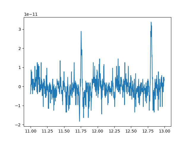
To illustrate the above two points, let’s select a couple seconds of data from the first channel:
sampling_freq = raw.info["sfreq"]
start_stop_seconds = np.array([11, 13])
start_sample, stop_sample = (start_stop_seconds * sampling_freq).astype(int)
channel_index = 0
raw_selection = raw[channel_index, start_sample:stop_sample]
print(raw_selection)
(array([[-3.85742192e-12, -3.85742192e-12, -9.64355481e-13, ...,
         2.89306644e-12,  3.85742192e-12,  3.85742192e-12]],
      shape=(1, 1201)), array([10.99872648, 11.00039144, 11.0020564 , ..., 12.9933487 ,
       12.99501366, 12.99667862], shape=(1201,)))
You can see that it contains 2 arrays. This combination of data and times
makes it easy to plot selections of raw data (although note that we’re
transposing the data array so that each channel is a column instead of a row,
to match what matplotlib expects when plotting 2-dimensional y against
1-dimensional x):
x = raw_selection[1]
y = raw_selection[0].T
plt.plot(x, y)
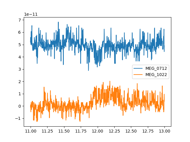
Extracting channels by name#
The Raw object can also be indexed with the names of
channels instead of their index numbers. You can pass a single string to get
just one channel, or a list of strings to select multiple channels. As with
integer indexing, this will return a tuple of (data_array, times_array)
that can be easily plotted. Since we’re plotting 2 channels this time, we’ll
add a vertical offset to one channel so it’s not plotted right on top
of the other one:
channel_names = ["MEG_0712", "MEG_1022"]
two_meg_chans = raw[channel_names, start_sample:stop_sample]
y_offset = np.array([5e-11, 0])  # just enough to separate the channel traces
x = two_meg_chans[1]
y = two_meg_chans[0].T + y_offset
lines = plt.plot(x, y)
plt.legend(lines, channel_names)
Extracting channels by type#
There are several ways to select all channels of a given type from a
Raw object. The safest method is to use
mne.pick_types() to obtain the integer indices of the channels you
want, then use those indices with the square-bracket indexing method shown
above. The pick_types() function uses the Info
attribute of the Raw object to determine channel types, and
takes boolean or string parameters to indicate which type(s) to retain. The
meg parameter defaults to True, and all others default to False,
so to get just the EEG channels, we pass eeg=True and meg=False:
eeg_channel_indices = mne.pick_types(raw.info, meg=False, eeg=True)
eeg_data, times = raw[eeg_channel_indices]
print(eeg_data.shape)
(58, 36038)
Some of the parameters of mne.pick_types() accept string arguments as
well as booleans. For example, the meg parameter can take values
'mag', 'grad', 'planar1', or 'planar2' to select only
magnetometers, all gradiometers, or a specific type of gradiometer. See the
docstring of mne.pick_types() for full details.
The Raw.get_data() method#
If you only want the data (not the corresponding array of times),
Raw objects have a get_data() method. Used
with no parameters specified, it will extract all data from all channels, in
a (n_channels, n_timepoints) NumPy array:
data = raw.get_data()
print(data.shape)
(376, 36038)
If you want the array of times, get_data() has an optional
return_times parameter:
data, times = raw.get_data(return_times=True)
print(data.shape)
print(times.shape)
(376, 36038)
(36038,)
The get_data() method can also be used to extract specific
channel(s) and sample ranges, via its picks, start, and stop
parameters. The picks parameter accepts integer channel indices, channel
names, or channel types, and preserves the requested channel order given as
its picks parameter.
first_channel_data = raw.get_data(picks=0)
eeg_and_eog_data = raw.get_data(picks=["eeg", "eog"])
two_meg_chans_data = raw.get_data(picks=["MEG_0712", "MEG_1022"], start=1000, stop=2000)

print(first_channel_data.shape)
print(eeg_and_eog_data.shape)
print(two_meg_chans_data.shape)
(1, 36038)
(61, 36038)
(2, 1000)
Summary of ways to extract data from Raw objects#
The following table summarizes the various ways of extracting data from a
Raw object.
Python code |
Result |
|---|---|
|
|
|
|
|
|
|
|
|
|
|
|
|
|
|
|
|
|
|
Exporting and saving Raw objects#
Raw objects have a built-in save() method,
which can be used to write a partially processed Raw object
to disk as a .fif file, such that it can be re-loaded later with its
various attributes intact (but see Floating-point precision for an important
note about numerical precision when saving).
There are a few other ways to export just the sensor data from a
Raw object. One is to use indexing or the
get_data() method to extract the data, and use
numpy.save() to save the data array:
data = raw.get_data()
np.save(file="my_data.npy", arr=data)
It is also possible to export the data to a Pandas DataFrame object, and use the saving methods that Pandas affords. The Raw object’s
to_data_frame() method is similar to
get_data() in that it has a picks parameter for
restricting which channels are exported, and start and stop
parameters for restricting the time domain. Note that, by default, times will
be converted to milliseconds, rounded to the nearest millisecond, and used as
the DataFrame index; see the scaling_time parameter in the documentation
of to_data_frame() for more details.
sampling_freq = raw.info["sfreq"]
start_end_secs = np.array([10, 13])
start_sample, stop_sample = (start_end_secs * sampling_freq).astype(int)
df = raw.to_data_frame(picks=["eeg"], start=start_sample, stop=stop_sample)
# then save using df.to_csv(...), df.to_hdf(...), etc
print(df.head())
        time       EEG_002  ...       EEG_059       EEG_060
0   9.999750  3.847885e+08  ...  5.243790e+08  6.952283e+08
1  10.001415  3.612900e+08  ...  5.200958e+08  7.069226e+08
2  10.003080  3.589401e+08  ...  5.176483e+08  7.080921e+08
3  10.004745  3.724518e+08  ...  5.182602e+08  7.010755e+08
4  10.006410  3.847885e+08  ...  5.286621e+08  7.069226e+08

[5 rows x 60 columns]
Note
When exporting data as a NumPy array or
Pandas DataFrame, be sure to properly account
for the unit of representation in your subsequent
analyses.
Total running time of the script: (0 minutes 1.916 seconds)