Cortical Signal Suppression (CSS) for removal of cortical signals

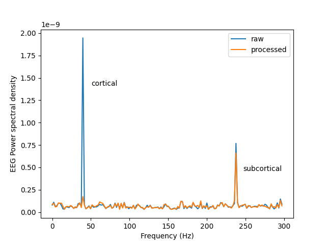
This script shows an example of how to use CSS [1] . CSS suppresses the cortical contribution to the signal subspace in EEG data using MEG data, facilitating detection of subcortical signals. We will illustrate how it works by simulating one cortical and one subcortical oscillation at different frequencies; 40 Hz and 239 Hz for cortical and subcortical activity, respectively, then process it with CSS and look at the power spectral density of the raw and processed data.

# Author: John G Samuelsson <johnsam@mit.edu>
# License: BSD-3-Clause
# Copyright the MNE-Python contributors.

import matplotlib.pyplot as plt
import numpy as np

import mne
from mne.datasets import sample
from mne.simulation import simulate_evoked, simulate_sparse_stc

Load sample subject data

data_path = sample.data_path()
subjects_dir = data_path / "subjects"
meg_path = data_path / "MEG" / "sample"
fwd_fname = meg_path / "sample_audvis-meg-eeg-oct-6-fwd.fif"
ave_fname = meg_path / "sample_audvis-no-filter-ave.fif"
cov_fname = meg_path / "sample_audvis-cov.fif"
trans_fname = meg_path / "sample_audvis_raw-trans.fif"
bem_fname = subjects_dir / "sample" / "bem" / "/sample-5120-bem-sol.fif"

raw = mne.io.read_raw_fif(meg_path / "sample_audvis_raw.fif")
fwd = mne.read_forward_solution(fwd_fname)
fwd = mne.convert_forward_solution(fwd, force_fixed=True, surf_ori=True)
fwd = mne.pick_types_forward(fwd, meg=True, eeg=True, exclude=raw.info["bads"])
cov = mne.read_cov(cov_fname)

Opening raw data file /home/circleci/mne_data/MNE-sample-data/MEG/sample/sample_audvis_raw.fif...
    Read a total of 3 projection items:
        PCA-v1 (1 x 102)  idle
        PCA-v2 (1 x 102)  idle
        PCA-v3 (1 x 102)  idle
    Range : 25800 ... 192599 =     42.956 ...   320.670 secs
Ready.
Reading forward solution from /home/circleci/mne_data/MNE-sample-data/MEG/sample/sample_audvis-meg-eeg-oct-6-fwd.fif...
    Reading a source space...
    Computing patch statistics...
    Patch information added...
    Distance information added...
    [done]
    Reading a source space...
    Computing patch statistics...
    Patch information added...
    Distance information added...
    [done]
    2 source spaces read
    Desired named matrix (kind = 3523) not available
    Read MEG forward solution (7498 sources, 306 channels, free orientations)
    Desired named matrix (kind = 3523) not available
    Read EEG forward solution (7498 sources, 60 channels, free orientations)
    Forward solutions combined: MEG, EEG
    Source spaces transformed to the forward solution coordinate frame
    Average patch normals will be employed in the rotation to the local surface coordinates....
    Converting to surface-based source orientations...
    [done]
    364 out of 366 channels remain after picking
    366 x 366 full covariance (kind = 1) found.
    Read a total of 4 projection items:
        PCA-v1 (1 x 102) active
        PCA-v2 (1 x 102) active
        PCA-v3 (1 x 102) active
        Average EEG reference (1 x 60) active

Find patches (labels) to activate

all_labels = mne.read_labels_from_annot(subject="sample", subjects_dir=subjects_dir)
labels = []
for select_label in ["parahippocampal-lh", "postcentral-rh"]:
    labels.append([lab for lab in all_labels if lab.name in select_label][0])
hiplab, postcenlab = labels

Reading labels from parcellation...
   read 34 labels from /home/circleci/mne_data/MNE-sample-data/subjects/sample/label/lh.aparc.annot
   read 34 labels from /home/circleci/mne_data/MNE-sample-data/subjects/sample/label/rh.aparc.annot

Simulate one cortical dipole (40 Hz) and one subcortical (239 Hz)

def cortical_waveform(times):
    """Create a cortical waveform."""
    return 10e-9 * np.cos(times * 2 * np.pi * 40)


def subcortical_waveform(times):
    """Create a subcortical waveform."""
    return 10e-9 * np.cos(times * 2 * np.pi * 239)


times = np.linspace(0, 0.5, int(0.5 * raw.info["sfreq"]))
stc = simulate_sparse_stc(
    fwd["src"],
    n_dipoles=2,
    times=times,
    location="center",
    subjects_dir=subjects_dir,
    labels=[postcenlab, hiplab],
    data_fun=cortical_waveform,
)
stc.data[np.where(np.isin(stc.vertices[0], hiplab.vertices))[0], :] = (
    subcortical_waveform(times)
)
evoked = simulate_evoked(fwd, stc, raw.info, cov, nave=15)

Projecting source estimate to sensor space...
[done]
4 projection items deactivated
Created an SSP operator (subspace dimension = 4)
4 projection items activated
SSP projectors applied...

Process with CSS and plot PSD of EEG data before and after processing

evoked_subcortical = mne.preprocessing.cortical_signal_suppression(evoked, n_proj=6)
chs = mne.pick_types(evoked.info, meg=False, eeg=True)

psd = np.mean(np.abs(np.fft.rfft(evoked.data)) ** 2, axis=0)
psd_proc = np.mean(np.abs(np.fft.rfft(evoked_subcortical.data)) ** 2, axis=0)
freq = np.arange(
    0, stop=int(evoked.info["sfreq"] / 2), step=evoked.info["sfreq"] / (2 * len(psd))
)

fig, ax = plt.subplots()
ax.plot(freq, psd, label="raw")
ax.plot(freq, psd_proc, label="processed")
ax.text(0.2, 0.7, "cortical", transform=ax.transAxes)
ax.text(0.8, 0.25, "subcortical", transform=ax.transAxes)
ax.set(ylabel="EEG Power spectral density", xlabel="Frequency (Hz)")
ax.legend()

# References
# ^^^^^^^^^^
#
# .. footbibliography::

Estimated memory usage: 141 MB