Note
Go to the end to download the full example code.
Compute MNE inverse solution on evoked data with a mixed source space#
Create a mixed source space and compute an MNE inverse solution on an evoked dataset.
# Author: Annalisa Pascarella <a.pascarella@iac.cnr.it>
#
# License: BSD-3-Clause
# Copyright the MNE-Python contributors.
import matplotlib.pyplot as plt
from nilearn import plotting

import mne
from mne.minimum_norm import apply_inverse, make_inverse_operator

# Set dir
data_path = mne.datasets.sample.data_path()
subject = "sample"
data_dir = data_path / "MEG" / subject
subjects_dir = data_path / "subjects"
bem_dir = subjects_dir / subject / "bem"

# Set file names
fname_mixed_src = bem_dir / f"{subject}-oct-6-mixed-src.fif"
fname_aseg = subjects_dir / subject / "mri" / "aseg.mgz"

fname_model = bem_dir / f"{subject}-5120-bem.fif"
fname_bem = bem_dir / f"{subject}-5120-bem-sol.fif"

fname_evoked = data_dir / f"{subject}_audvis-ave.fif"
fname_trans = data_dir / f"{subject}_audvis_raw-trans.fif"
fname_fwd = data_dir / f"{subject}_audvis-meg-oct-6-mixed-fwd.fif"
fname_cov = data_dir / f"{subject}_audvis-shrunk-cov.fif"
Set up our source space#
List substructures we are interested in. We select only the sub structures we want to include in the source space:
labels_vol = [
    "Left-Amygdala",
    "Left-Thalamus-Proper",
    "Left-Cerebellum-Cortex",
    "Brain-Stem",
    "Right-Amygdala",
    "Right-Thalamus-Proper",
    "Right-Cerebellum-Cortex",
]
Get a surface-based source space, here with few source points for speed in this demonstration, in general you should use oct6 spacing!
src = mne.setup_source_space(
    subject, spacing="oct5", add_dist=False, subjects_dir=subjects_dir
)
Setting up the source space with the following parameters:

SUBJECTS_DIR = /home/circleci/mne_data/MNE-sample-data/subjects
Subject      = sample
Surface      = white
Octahedron subdivision grade 5

>>> 1. Creating the source space...

Doing the octahedral vertex picking...
Loading /home/circleci/mne_data/MNE-sample-data/subjects/sample/surf/lh.white...
Mapping lh sample -> oct (5) ...
    Triangle neighbors and vertex normals...
Loading geometry from /home/circleci/mne_data/MNE-sample-data/subjects/sample/surf/lh.sphere...
Setting up the triangulation for the decimated surface...
loaded lh.white 1026/155407 selected to source space (oct = 5)

Loading /home/circleci/mne_data/MNE-sample-data/subjects/sample/surf/rh.white...
Mapping rh sample -> oct (5) ...
    Triangle neighbors and vertex normals...
Loading geometry from /home/circleci/mne_data/MNE-sample-data/subjects/sample/surf/rh.sphere...
Setting up the triangulation for the decimated surface...
loaded rh.white 1026/156866 selected to source space (oct = 5)

You are now one step closer to computing the gain matrix
Now we create a mixed src space by adding the volume regions specified in the list labels_vol. First, read the aseg file and the source space bounds using the inner skull surface (here using 10mm spacing to save time, we recommend something smaller like 5.0 in actual analyses):
vol_src = mne.setup_volume_source_space(
    subject,
    mri=fname_aseg,
    pos=10.0,
    bem=fname_model,
    volume_label=labels_vol,
    subjects_dir=subjects_dir,
    add_interpolator=False,  # just for speed, usually this should be True
    verbose=True,
)

# Generate the mixed source space
src += vol_src
print(
    f"The source space contains {len(src)} spaces and "
    f"{sum(s['nuse'] for s in src)} vertices"
)
BEM              : /home/circleci/mne_data/MNE-sample-data/subjects/sample/bem/sample-5120-bem.fif
grid                  : 10.0 mm
mindist               : 5.0 mm
MRI volume            : /home/circleci/mne_data/MNE-sample-data/subjects/sample/mri/aseg.mgz

Reading /home/circleci/mne_data/MNE-sample-data/subjects/sample/mri/aseg.mgz...

Loaded inner skull from /home/circleci/mne_data/MNE-sample-data/subjects/sample/bem/sample-5120-bem.fif (2562 nodes)
Surface CM = (   0.7  -10.0   44.3) mm
Surface fits inside a sphere with radius   91.8 mm
Surface extent:
    x =  -66.7 ...   68.8 mm
    y =  -88.0 ...   79.0 mm
    z =  -44.5 ...  105.8 mm
Grid extent:
    x =  -70.0 ...   70.0 mm
    y =  -90.0 ...   80.0 mm
    z =  -50.0 ...  110.0 mm
4590 sources before omitting any.
2961 sources after omitting infeasible sources not within 0.0 - 91.8 mm.
Source spaces are in MRI coordinates.
Checking that the sources are inside the surface and at least    5.0 mm away (will take a few...)
Checking surface interior status for 2961 points...
    Found  346/2961 points inside  an interior sphere of radius   43.6 mm
    Found    0/2961 points outside an exterior sphere of radius   91.8 mm
    Found 1275/2615 points outside using surface Qhull
    Found   97/1340 points outside using solid angles
    Total 1589/2961 points inside the surface
Interior check completed in 252.5 ms
    1372 source space points omitted because they are outside the inner skull surface.
    283 source space points omitted because of the    5.0-mm distance limit.
1306 sources remaining after excluding the sources outside the surface and less than    5.0 mm inside.
    Selected 2 voxels from Left-Amygdala
    Selected 9 voxels from Left-Thalamus-Proper
    Selected 33 voxels from Left-Cerebellum-Cortex
    Selected 21 voxels from Brain-Stem
    Selected 1 voxel from Right-Amygdala
    Selected 7 voxels from Right-Thalamus-Proper
    Selected 44 voxels from Right-Cerebellum-Cortex
Adjusting the neighborhood info.
Source space : MRI voxel -> MRI (surface RAS)
    0.010000 0.000000 0.000000     -70.00 mm
    0.000000 0.010000 0.000000     -90.00 mm
    0.000000 0.000000 0.010000     -50.00 mm
    0.000000 0.000000 0.000000       1.00
MRI volume : MRI voxel -> MRI (surface RAS)
    -0.001000 0.000000 0.000000     128.00 mm
    0.000000 0.000000 0.001000    -128.00 mm
    0.000000 -0.001000 0.000000     128.00 mm
    0.000000 0.000000 0.000000       1.00
MRI volume : MRI (surface RAS) -> RAS (non-zero origin)
    1.000000 -0.000000 -0.000000      -5.27 mm
    -0.000000 1.000000 -0.000000       9.04 mm
    -0.000000 0.000000 1.000000     -27.29 mm
    0.000000 0.000000 0.000000       1.00
The source space contains 9 spaces and 2169 vertices
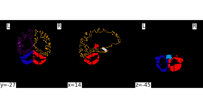
View the source space#
We could write the mixed source space with:
>>> write_source_spaces(fname_mixed_src, src, overwrite=True)
We can also export source positions to NIfTI file and visualize it again:
nii_fname = bem_dir / f"{subject}-mixed-src.nii"
src.export_volume(nii_fname, mri_resolution=True, overwrite=True)
plotting.plot_img(str(nii_fname), cmap="nipy_spectral")
Reading FreeSurfer lookup table
Compute the fwd matrix#
fwd = mne.make_forward_solution(
    fname_evoked,
    fname_trans,
    src,
    fname_bem,
    mindist=5.0,  # ignore sources<=5mm from innerskull
    meg=True,
    eeg=False,
    n_jobs=None,
)
del src  # save memory

leadfield = fwd["sol"]["data"]
ns, nd = leadfield.shape
print(f"Leadfield size : {ns} sensors x {nd} dipoles")
print(
    f"The fwd source space contains {len(fwd['src'])} spaces and "
    f"{sum(s['nuse'] for s in fwd['src'])} vertices"
)

# Load data
condition = "Left Auditory"
evoked = mne.read_evokeds(fname_evoked, condition=condition, baseline=(None, 0))
noise_cov = mne.read_cov(fname_cov)
Source space          : <SourceSpaces: [<surface (lh), n_vertices=155407, n_used=1026>, <surface (rh), n_vertices=156866, n_used=1026>, <volume (Left-Amygdala), n_used=2>, <volume (Left-Thalamus-Proper), n_used=9>, <volume (Left-Cerebellum-Cortex), n_used=33>, <volume (Brain-Stem), n_used=21>, <volume (Right-Amygdala), n_used=1>, <volume (Right-Thalamus-Proper), n_used=7>, <volume (Right-Cerebellum-Cortex), n_used=44>] MRI (surface RAS) coords, subject 'sample', ~30.5 MiB>
MRI -> head transform : /home/circleci/mne_data/MNE-sample-data/MEG/sample/sample_audvis_raw-trans.fif
Measurement data      : sample_audvis-ave.fif
Conductor model   : /home/circleci/mne_data/MNE-sample-data/subjects/sample/bem/sample-5120-bem-sol.fif
Accurate field computations
Do computations in head coordinates
Free source orientations

Read 9 source spaces a total of 2169 active source locations

Coordinate transformation: MRI (surface RAS) -> head
    0.999310 0.009985 -0.035787      -3.17 mm
    0.012759 0.812405 0.582954       6.86 mm
    0.034894 -0.583008 0.811716      28.88 mm
    0.000000 0.000000 0.000000       1.00

Read 306 MEG channels from info
105 coil definitions read
Coordinate transformation: MEG device -> head
    0.991420 -0.039936 -0.124467      -6.13 mm
    0.060661 0.984012 0.167456       0.06 mm
    0.115790 -0.173570 0.977991      64.74 mm
    0.000000 0.000000 0.000000       1.00
MEG coil definitions created in head coordinates.
Source spaces are now in head coordinates.

Setting up the BEM model using /home/circleci/mne_data/MNE-sample-data/subjects/sample/bem/sample-5120-bem-sol.fif...

Loading surfaces...

Loading the solution matrix...

Homogeneous model surface loaded.
Loaded linear collocation BEM solution from /home/circleci/mne_data/MNE-sample-data/subjects/sample/bem/sample-5120-bem-sol.fif
Employing the head->MRI coordinate transform with the BEM model.
BEM model sample-5120-bem-sol.fif is now set up


Source spaces are in head coordinates.
Checking that the sources are inside the surface and at least    5.0 mm away (will take a few...)
Checking surface interior status for 1026 points...
    Found  211/1026 points inside  an interior sphere of radius   43.6 mm
    Found    0/1026 points outside an exterior sphere of radius   91.8 mm
    Found    0/ 815 points outside using surface Qhull
    Found    0/ 815 points outside using solid angles
    Total 1026/1026 points inside the surface
Interior check completed in 123.9 ms
    84 source space point omitted because of the    5.0-mm distance limit.
Checking surface interior status for 1026 points...
    Found  219/1026 points inside  an interior sphere of radius   43.6 mm
    Found    0/1026 points outside an exterior sphere of radius   91.8 mm
    Found    0/ 807 points outside using surface Qhull
    Found    0/ 807 points outside using solid angles
    Total 1026/1026 points inside the surface
Interior check completed in 126.5 ms
    84 source space point omitted because of the    5.0-mm distance limit.
Checking surface interior status for 2 points...
    Found 2/2 points inside  an interior sphere of radius   43.6 mm
    Found 0/2 points outside an exterior sphere of radius   91.8 mm
    Found 0/0 points outside using surface Qhull
    Found 0/0 points outside using solid angles
    Total 2/2 points inside the surface
Interior check completed in 1.1 ms
Checking surface interior status for 9 points...
    Found 9/9 points inside  an interior sphere of radius   43.6 mm
    Found 0/9 points outside an exterior sphere of radius   91.8 mm
    Found 0/0 points outside using surface Qhull
    Found 0/0 points outside using solid angles
    Total 9/9 points inside the surface
Interior check completed in 1.0 ms
Checking surface interior status for 33 points...
    Found  1/33 point  inside  an interior sphere of radius   43.6 mm
    Found  0/33 points outside an exterior sphere of radius   91.8 mm
    Found  0/32 points outside using surface Qhull
    Found  0/32 points outside using solid angles
    Total 33/33 points inside the surface
Interior check completed in 7.0 ms
Checking surface interior status for 21 points...
    Found  8/21 points inside  an interior sphere of radius   43.6 mm
    Found  0/21 points outside an exterior sphere of radius   91.8 mm
    Found  0/13 points outside using surface Qhull
    Found  0/13 points outside using solid angles
    Total 21/21 points inside the surface
Interior check completed in 3.0 ms
Checking surface interior status for 1 point ...
    Found 1/1 point  inside  an interior sphere of radius   43.6 mm
    Found 0/1 points outside an exterior sphere of radius   91.8 mm
    Found 0/0 points outside using surface Qhull
    Found 0/0 points outside using solid angles
    Total 1/1 point  inside the surface
Interior check completed in 0.8 ms
Checking surface interior status for 7 points...
    Found 7/7 points inside  an interior sphere of radius   43.6 mm
    Found 0/7 points outside an exterior sphere of radius   91.8 mm
    Found 0/0 points outside using surface Qhull
    Found 0/0 points outside using solid angles
    Total 7/7 points inside the surface
Interior check completed in 0.9 ms
Checking surface interior status for 44 points...
    Found  1/44 point  inside  an interior sphere of radius   43.6 mm
    Found  0/44 points outside an exterior sphere of radius   91.8 mm
    Found  0/43 points outside using surface Qhull
    Found  0/43 points outside using solid angles
    Total 44/44 points inside the surface
Interior check completed in 7.8 ms
Checking surface interior status for 306 points...
    Found   0/306 points inside  an interior sphere of radius   43.6 mm
    Found 306/306 points outside an exterior sphere of radius   91.8 mm
    Found   0/  0 points outside using surface Qhull
    Found   0/  0 points outside using solid angles
    Total 0/306 points inside the surface
Interior check completed in 1.0 ms

Composing the field computation matrix...
Computing MEG at 2001 source locations (free orientations)...

Finished.
Leadfield size : 306 sensors x 6003 dipoles
The fwd source space contains 9 spaces and 2001 vertices
Reading /home/circleci/mne_data/MNE-sample-data/MEG/sample/sample_audvis-ave.fif ...
    Read a total of 4 projection items:
        PCA-v1 (1 x 10²) active
        PCA-v2 (1 x 10²) active
        PCA-v3 (1 x 10²) active
        Average EEG reference (1 x 60) active
    Found the data of interest:
        t =    -199.80 ...     499.49 ms (Left Auditory)
        0 CTF compensation matrices available
        nave = 55 - aspect type = 100
Projections have already been applied. Setting proj attribute to True.
Applying baseline correction (mode: mean)
    365 x 365 full covariance (kind = 1) found.
    Read a total of 4 projection items:
        PCA-v1 (1 x 10²) active
        PCA-v2 (1 x 10²) active
        PCA-v3 (1 x 10²) active
        Average EEG reference (1 x 59) active
Compute inverse solution#
snr = 3.0  # use smaller SNR for raw data
inv_method = "dSPM"  # sLORETA, MNE, dSPM
parc = "aparc"  # the parcellation to use, e.g., 'aparc' 'aparc.a2009s'
loose = dict(surface=0.2, volume=1.0)

lambda2 = 1.0 / snr**2

inverse_operator = make_inverse_operator(
    evoked.info, fwd, noise_cov, depth=None, loose=loose, verbose=True
)
del fwd

stc = apply_inverse(evoked, inverse_operator, lambda2, inv_method, pick_ori=None)
src = inverse_operator["src"]
Converting forward solution to surface orientation
    No patch info available. The standard source space normals will be employed in the rotation to the local surface coordinates....
    Converting to surface-based source orientations...
    [done]
info["bads"] and noise_cov["bads"] do not match, excluding bad channels from both
Computing inverse operator with 305 channels.
    305 out of 306 channels remain after picking
Selected 305 channels
Applying loose dipole orientations to surface source spaces: 0.2
Applying free  dipole orientations to volume  source spaces: 1.0
Whitening the forward solution.
    Created an SSP operator (subspace dimension = 3)
Computing rank from covariance with rank=None
    Using tolerance 3.5e-13 (2.2e-16 eps * 305 dim * 5.2  max singular value)
    Estimated rank (mag + grad): 302
    MEG: rank 302 computed from 305 data channels with 3 projectors
    Setting small MEG eigenvalues to zero (without PCA)
Creating the source covariance matrix
Adjusting source covariance matrix.
Computing SVD of whitened and weighted lead field matrix.
    largest singular value = 4.39266
    scaling factor to adjust the trace = 3.01344e+19 (nchan = 305 nzero = 3)
Preparing the inverse operator for use...
    Scaled noise and source covariance from nave = 1 to nave = 55
    Created the regularized inverter
    Created an SSP operator (subspace dimension = 3)
    Created the whitener using a noise covariance matrix with rank 302 (3 small eigenvalues omitted)
    Computing noise-normalization factors (dSPM)...
[done]
Applying inverse operator to "Left Auditory"...
    Picked 305 channels from the data
    Computing inverse...
    Eigenleads need to be weighted ...
    Computing residual...
    Explained  59.0% variance
    Combining the current components...
    dSPM...
[done]
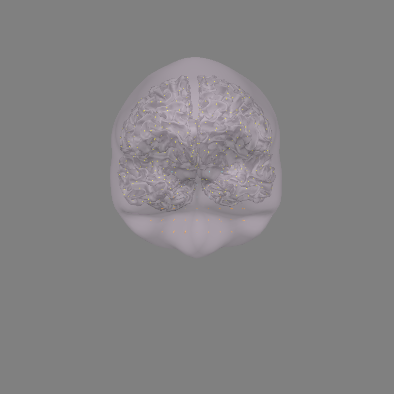
Plot the mixed source estimate#
initial_time = 0.1
stc_vec = apply_inverse(
    evoked, inverse_operator, lambda2, inv_method, pick_ori="vector"
)
brain = stc_vec.plot(
    hemi="both",
    src=inverse_operator["src"],
    views="coronal",
    initial_time=initial_time,
    subjects_dir=subjects_dir,
    brain_kwargs=dict(silhouette=True),
    smoothing_steps=7,
)
Preparing the inverse operator for use...
    Scaled noise and source covariance from nave = 1 to nave = 55
    Created the regularized inverter
    Created an SSP operator (subspace dimension = 3)
    Created the whitener using a noise covariance matrix with rank 302 (3 small eigenvalues omitted)
    Computing noise-normalization factors (dSPM)...
[done]
Applying inverse operator to "Left Auditory"...
    Picked 305 channels from the data
    Computing inverse...
    Eigenleads need to be weighted ...
    Computing residual...
    Explained  59.0% variance
    dSPM...
[done]
Using control points [ 3.43101017  3.98225664 16.7504814 ]
    Triangle neighbors and vertex normals...
Loading geometry from /home/circleci/mne_data/MNE-sample-data/subjects/sample/surf/lh.sphere...
Setting up the triangulation for the decimated surface...
    Triangle neighbors and vertex normals...
Loading geometry from /home/circleci/mne_data/MNE-sample-data/subjects/sample/surf/rh.sphere...
Setting up the triangulation for the decimated surface...
Plot the surface#
brain = stc.surface().plot(
    initial_time=initial_time, subjects_dir=subjects_dir, smoothing_steps=7
)
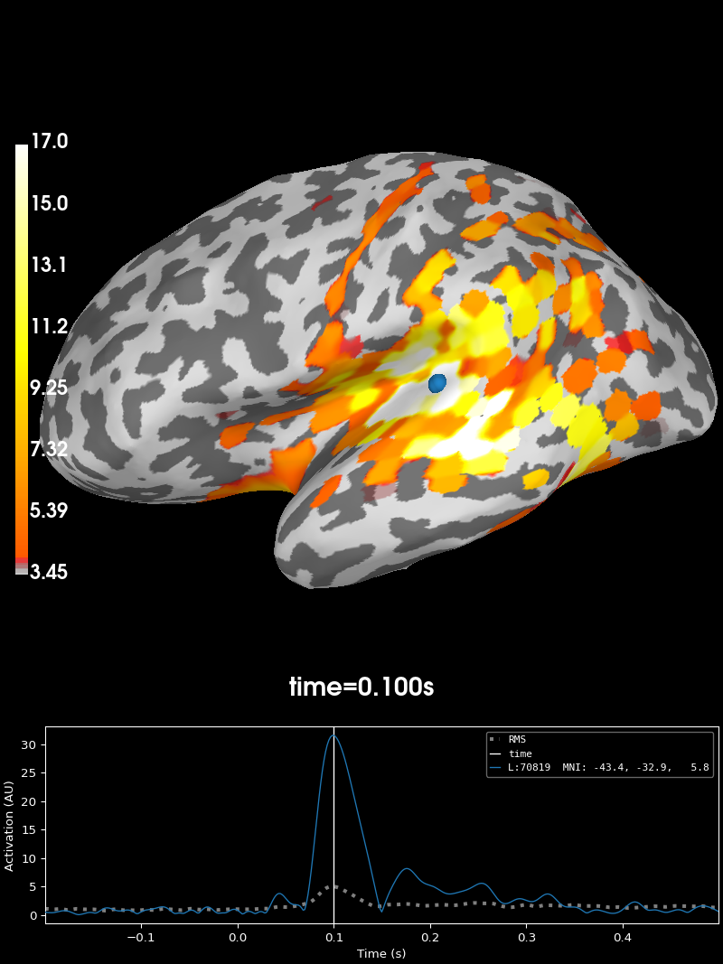
Using control points [ 3.45409596 4.02821048 16.97219252]
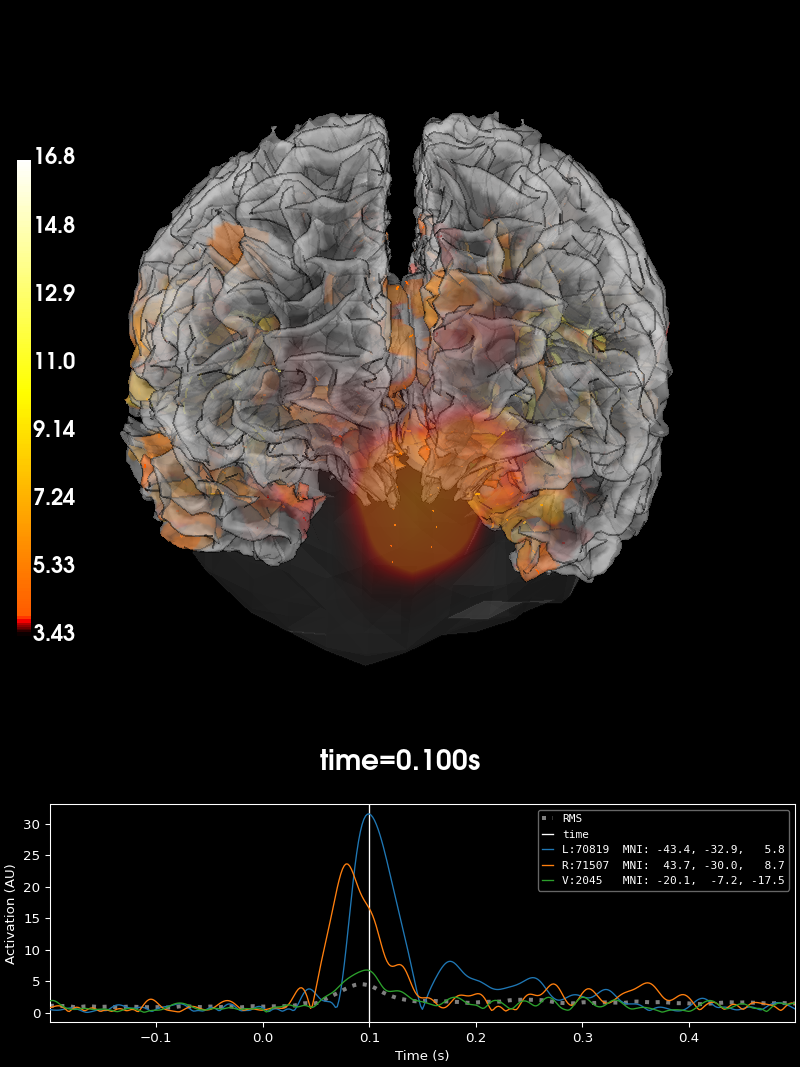
Plot the volume#
fig = stc.volume().plot(initial_time=initial_time, src=src, subjects_dir=subjects_dir)
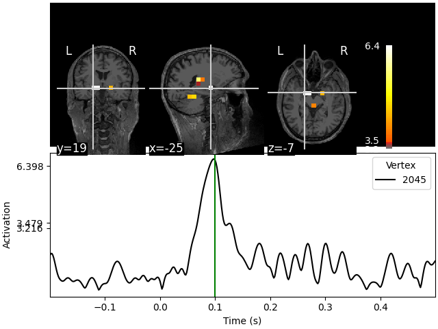
Fixing initial time: 0.1 s
Showing: t = 0.100 s, (-25.3, 19.0, -7.3) mm, [5, 10, 7] vox, 2045 vertex
Using control points [3.21567156 3.47889133 6.39837939]
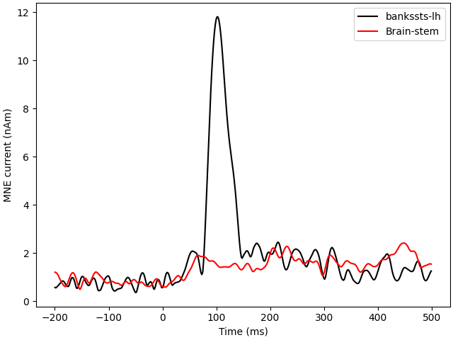
Process labels#
Average the source estimates within each label of the cortical parcellation and each sub structure contained in the src space
# Get labels for FreeSurfer 'aparc' cortical parcellation with 34 labels/hemi
labels_parc = mne.read_labels_from_annot(subject, parc=parc, subjects_dir=subjects_dir)

label_ts = mne.extract_label_time_course(
    [stc], labels_parc, src, mode="mean", allow_empty=True
)

# plot the times series of 2 labels
fig, axes = plt.subplots(1, layout="constrained")
axes.plot(1e3 * stc.times, label_ts[0][0, :], "k", label="bankssts-lh")
axes.plot(1e3 * stc.times, label_ts[0][-1, :].T, "r", label="Brain-stem")
axes.set(xlabel="Time (ms)", ylabel="MNE current (nAm)")
axes.legend()
Reading labels from parcellation...
   read 34 labels from /home/circleci/mne_data/MNE-sample-data/subjects/sample/label/lh.aparc.annot
   read 34 labels from /home/circleci/mne_data/MNE-sample-data/subjects/sample/label/rh.aparc.annot
Extracting time courses for 75 labels (mode: mean)
Total running time of the script: (0 minutes 44.496 seconds)