Plotting topographic maps of evoked data

Load evoked data and plot topomaps for selected time points using multiple additional options.

# Authors: Christian Brodbeck <christianbrodbeck@nyu.edu>
#          Tal Linzen <linzen@nyu.edu>
#          Denis A. Engeman <denis.engemann@gmail.com>
#          Mikołaj Magnuski <mmagnuski@swps.edu.pl>
#          Eric Larson <larson.eric.d@gmail.com>
#          Alex Rockhill <aprockhill@mailbox.org>
#
# License: BSD-3-Clause
# Copyright the MNE-Python contributors.

sphinx_gallery_thumbnail_number = 5

import matplotlib.pyplot as plt
import numpy as np

from mne import read_evokeds
from mne.datasets import sample

print(__doc__)

path = sample.data_path()
fname = path / "MEG" / "sample" / "sample_audvis-ave.fif"

# load evoked corresponding to a specific condition
# from the fif file and subtract baseline
condition = "Left Auditory"
evoked = read_evokeds(fname, condition=condition, baseline=(None, 0))

Reading /home/circleci/mne_data/MNE-sample-data/MEG/sample/sample_audvis-ave.fif ...
    Read a total of 4 projection items:
        PCA-v1 (1 x 102) active
        PCA-v2 (1 x 102) active
        PCA-v3 (1 x 102) active
        Average EEG reference (1 x 60) active
    Found the data of interest:
        t =    -199.80 ...     499.49 ms (Left Auditory)
        0 CTF compensation matrices available
        nave = 55 - aspect type = 100
Projections have already been applied. Setting proj attribute to True.
Applying baseline correction (mode: mean)

Basic plot_topomap() options

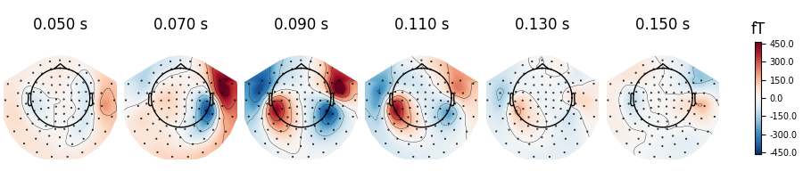
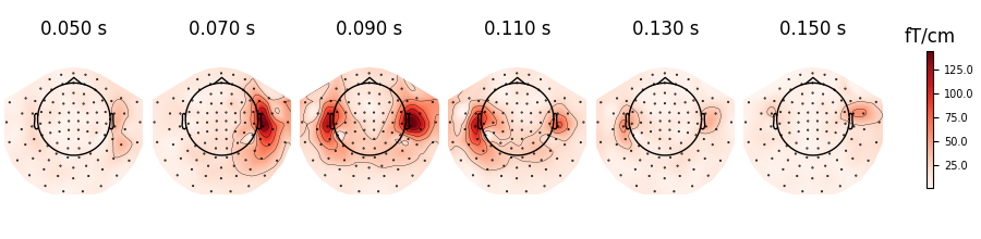
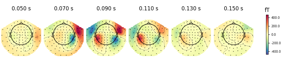
We plot evoked topographies using mne.Evoked.plot_topomap(). The first argument, times allows to specify time instants (in seconds!) for which topographies will be shown. We select timepoints from 50 to 150 ms with a step of 20ms and plot magnetometer data:

times = np.arange(0.05, 0.151, 0.02)
evoked.plot_topomap(times, ch_type="mag")

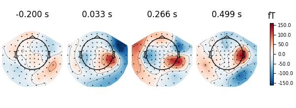
If times is set to None at most 10 regularly spaced topographies will be shown:

evoked.plot_topomap(ch_type="mag")

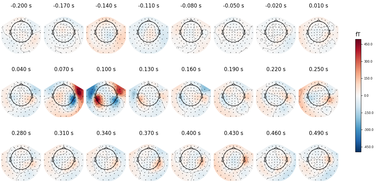
We can use nrows and ncols parameter to create multiline plots with more timepoints.

all_times = np.arange(-0.2, 0.5, 0.03)
evoked.plot_topomap(all_times, ch_type="mag", ncols=8, nrows="auto")

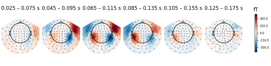
Instead of showing topographies at specific time points we can compute averages of 50 ms bins centered on these time points to reduce the noise in the topographies:

evoked.plot_topomap(times, ch_type="mag", average=0.05)

We can plot gradiometer data (plots the RMS for each pair of gradiometers)

evoked.plot_topomap(times, ch_type="grad")

Additional plot_topomap() options

We can also use a range of various mne.viz.plot_topomap() arguments that control how the topography is drawn. For example:

• cmap - to specify the color map

• res - to control the resolution of the topographies (lower resolution means faster plotting)

• contours to define how many contour lines should be plotted

evoked.plot_topomap(times, ch_type="mag", cmap="Spectral_r", res=32, contours=4)

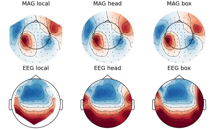
If you look at the edges of the head circle of a single topomap you’ll see the effect of extrapolation. There are three extrapolation modes:

• extrapolate='local' extrapolates only to points close to the sensors.

• extrapolate='head' extrapolates out to the head circle.

• extrapolate='box' extrapolates to a large box stretching beyond the head circle.

The default value extrapolate='auto' will use 'local' for MEG sensors and 'head' otherwise. Here we show each option:

extrapolations = ["local", "head", "box"]
fig, axes = plt.subplots(figsize=(7.5, 4.5), nrows=2, ncols=3, layout="constrained")

# Here we look at EEG channels, and use a custom head sphere to get all the
# sensors to be well within the drawn head surface
for axes_row, ch_type in zip(axes, ("mag", "eeg")):
    for ax, extr in zip(axes_row, extrapolations):
        evoked.plot_topomap(
            0.1,
            ch_type=ch_type,
            size=2,
            extrapolate=extr,
            axes=ax,
            show=False,
            colorbar=False,
            sphere=(0.0, 0.0, 0.0, 0.09),
        )
        ax.set_title(f"{ch_type.upper()} {extr}", fontsize=14)

More advanced usage

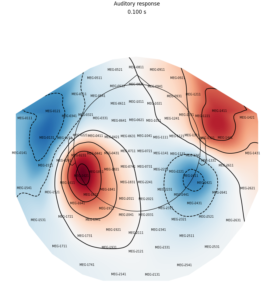
Now we plot magnetometer data as topomap at a single time point: 100 ms post-stimulus, add channel labels, title and adjust plot margins:

fig = evoked.plot_topomap(
    0.1, ch_type="mag", show_names=True, colorbar=False, size=6, res=128
)
fig.suptitle("Auditory response")

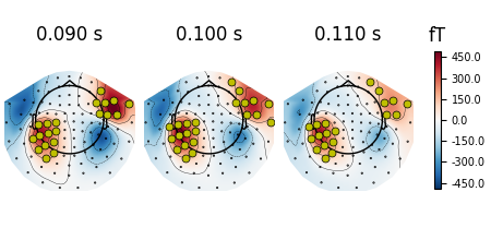
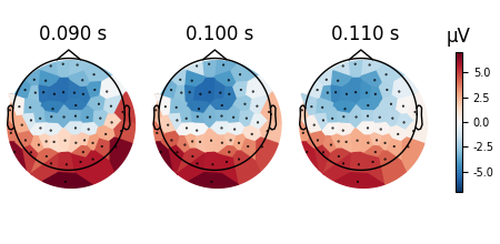
We can also highlight specific channels by adding a mask, to e.g. mark channels exceeding a threshold at a given time:

# Define a threshold and create the mask
mask = evoked.data > 1e-13

# Select times and plot
times = (0.09, 0.1, 0.11)
mask_params = dict(markersize=10, markerfacecolor="y")
evoked.plot_topomap(times, ch_type="mag", mask=mask, mask_params=mask_params)

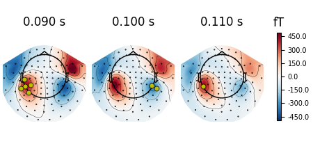
Or by manually picking the channels to highlight at different times:

times = (0.09, 0.1, 0.11)
_times = ((np.abs(evoked.times - t)).argmin() for t in times)
significant_channels = [
    ("MEG 0231", "MEG 1611", "MEG 1621", "MEG 1631", "MEG 1811"),
    ("MEG 2411", "MEG 2421"),
    ("MEG 1621"),
]
_channels = [np.isin(evoked.ch_names, ch) for ch in significant_channels]

mask = np.zeros(evoked.data.shape, dtype="bool")
for _chs, _time in zip(_channels, _times):
    mask[_chs, _time] = True

evoked.plot_topomap(times, ch_type="mag", mask=mask, mask_params=mask_params)

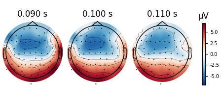
Interpolating topomaps

We can also look at the effects of interpolating our data. Perhaps, we might have data per channel such as the impedance of each electrode that we don’t want interpolated, or we just want to visualize the data without interpolation as a sanity check. We can use image_interp='nearest' to prevent any interpolation or image_interp='linear' to do a linear interpolation instead of the default cubic interpolation.

The default cubic interpolation is the smoothest and is great for publications.

evoked.plot_topomap(times, ch_type="eeg", image_interp="cubic")

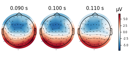
The linear interpolation might be helpful in some cases.

evoked.plot_topomap(times, ch_type="eeg", image_interp="linear")

The nearest (Voronoi, no interpolation) interpolation is especially helpful for debugging and seeing the values assigned to the topomap unaltered.

evoked.plot_topomap(times, ch_type="eeg", image_interp="nearest", contours=0)

Animating the topomap

Instead of using a still image we can plot magnetometer data as an animation, which animates properly only in matplotlib interactive mode.

times = np.arange(0.05, 0.151, 0.01)
fig, anim = evoked.animate_topomap(times=times, ch_type="mag", frame_rate=2, blit=False)

Estimated memory usage: 9 MB