Note
Go to the end to download the full example code.
Non-parametric 1 sample cluster statistic on single trial power#
This script shows how to estimate significant clusters in time-frequency power estimates. It uses a non-parametric statistical procedure based on permutations and cluster level statistics.
The procedure consists of:
extracting epochs
compute single trial power estimates
baseline line correct the power estimates (power ratios)
compute stats to see if ratio deviates from 1.
Here, the unit of observation is epochs from a specific study subject. However, the same logic applies when the unit of observation is a number of study subjects each of whom contribute their own averaged data (i.e., an average of their epochs). This would then be considered an analysis at the “2nd level”.
For more information on cluster-based permutation testing in MNE-Python, see also: Spatiotemporal permutation F-test on full sensor data.
# Authors: Alexandre Gramfort <alexandre.gramfort@inria.fr>
#          Stefan Appelhoff <stefan.appelhoff@mailbox.org>
#
# License: BSD-3-Clause
# Copyright the MNE-Python contributors.
import matplotlib.pyplot as plt
import numpy as np
import scipy.stats

import mne
from mne.datasets import sample
from mne.stats import permutation_cluster_1samp_test
Set parameters#
data_path = sample.data_path()
meg_path = data_path / "MEG" / "sample"
raw_fname = meg_path / "sample_audvis_raw.fif"
tmin, tmax, event_id = -0.3, 0.6, 1

# Setup for reading the raw data
raw = mne.io.read_raw_fif(raw_fname)
events = mne.find_events(raw, stim_channel="STI 014")

include = []
raw.info["bads"] += ["MEG 2443", "EEG 053"]  # bads + 2 more

# for speed, we'll only look at right-temporal gradiometers (and EOG)
picks_eog = mne.pick_types(raw.info, eog=True)
picks_grad = mne.pick_types(raw.info, meg="grad", exclude="bads")
picks_rtemp = mne.pick_channels(
    raw.info["ch_names"], mne.read_vectorview_selection("Right-temporal"), ordered=True
)
picks = list((set(picks_rtemp) & set(picks_grad)) | set(picks_eog))

# Load condition 1
event_id = 1
epochs = mne.Epochs(
    raw,
    events,
    event_id,
    tmin,
    tmax,
    picks=picks,
    baseline=(None, 0),
    preload=True,
    reject=dict(grad=4000e-13, eog=150e-6),
)

evoked = epochs.average()

# Factor to down-sample the temporal dimension of the TFR computed by
# tfr_morlet. Decimation occurs after frequency decomposition and can
# be used to reduce memory usage (and possibly computational time of downstream
# operations such as nonparametric statistics) if you don't need high
# spectrotemporal resolution.
decim = 5

# define frequencies of interest
freqs = np.arange(8, 40, 2)

# run the TFR decomposition
tfr_epochs = epochs.compute_tfr(
    "morlet",
    freqs,
    n_cycles=4.0,
    decim=decim,
    average=False,
    return_itc=False,
    n_jobs=None,
)

# Baseline power
tfr_epochs.apply_baseline(mode="logratio", baseline=(-0.100, 0))

# Crop in time to keep only what is between 0 and 400 ms
evoked.crop(-0.1, 0.4)
tfr_epochs.crop(-0.1, 0.4)

epochs_power = tfr_epochs.data
Opening raw data file /home/circleci/mne_data/MNE-sample-data/MEG/sample/sample_audvis_raw.fif...
    Read a total of 3 projection items:
        PCA-v1 (1 x 10²)  idle
        PCA-v2 (1 x 10²)  idle
        PCA-v3 (1 x 10²)  idle
    Range : 25800 ... 192599 =     42.956 ...   320.670 secs
Ready.
Finding events on: STI 014
320 events found on stim channel STI 014
Event IDs: [ 1  2  3  4  5 32]
Not setting metadata
72 matching events found
Setting baseline interval to [-0.2996928197375818, 0.0] s
Applying baseline correction (mode: mean)
0 projection items activated
Loading data for 72 events and 541 original time points ...
    Rejecting  epoch based on EOG : ['EOG 061']
    Rejecting  epoch based on EOG : ['EOG 061']
    Rejecting  epoch based on EOG : ['EOG 061']
    Rejecting  epoch based on EOG : ['EOG 061']
    Rejecting  epoch based on EOG : ['EOG 061']
    Rejecting  epoch based on EOG : ['EOG 061']
    Rejecting  epoch based on EOG : ['EOG 061']
    Rejecting  epoch based on EOG : ['EOG 061']
    Rejecting  epoch based on EOG : ['EOG 061']
    Rejecting  epoch based on EOG : ['EOG 061']
    Rejecting  epoch based on EOG : ['EOG 061']
    Rejecting  epoch based on EOG : ['EOG 061']
    Rejecting  epoch based on EOG : ['EOG 061']
    Rejecting  epoch based on EOG : ['EOG 061']
    Rejecting  epoch based on EOG : ['EOG 061']
    Rejecting  epoch based on EOG : ['EOG 061']
    Rejecting  epoch based on EOG : ['EOG 061']
    Rejecting  epoch based on EOG : ['EOG 061']
18 bad epochs dropped
Applying baseline correction (mode: logratio)
Define adjacency for statistics#
To perform a cluster-based permutation test, we need a suitable definition for the adjacency of sensors, time points, and frequency bins. The adjacency matrix will be used to form clusters.
We first compute the sensor adjacency, and then combine that with a “lattice” adjacency for the time-frequency plane, which assumes that elements at index “N” are adjacent to elements at indices “N + 1” and “N - 1” (forming a “grid” on the time-frequency plane).
# find_ch_adjacency first attempts to find an existing "neighbor"
# (adjacency) file for given sensor layout.
# If such a file doesn't exist, an adjacency matrix is computed on the fly,
# using Delaunay triangulations.
sensor_adjacency, ch_names = mne.channels.find_ch_adjacency(tfr_epochs.info, "grad")

# In this case, find_ch_adjacency finds an appropriate file and
# reads it (see log output: "neuromag306planar").
# However, we need to subselect the channels we are actually using
use_idx = [ch_names.index(ch_name) for ch_name in tfr_epochs.ch_names]
sensor_adjacency = sensor_adjacency[use_idx][:, use_idx]

# Our sensor adjacency matrix is of shape n_chs × n_chs
assert sensor_adjacency.shape == (len(tfr_epochs.ch_names), len(tfr_epochs.ch_names))

# Now we need to prepare adjacency information for the time-frequency
# plane. For that, we use "combine_adjacency", and pass dimensions
# as in the data we want to test (excluding observations). Here:
# channels × frequencies × times
assert epochs_power.data.shape == (
    len(epochs),
    len(tfr_epochs.ch_names),
    len(tfr_epochs.freqs),
    len(tfr_epochs.times),
)
adjacency = mne.stats.combine_adjacency(
    sensor_adjacency, len(tfr_epochs.freqs), len(tfr_epochs.times)
)

# The overall adjacency we end up with is a square matrix with each
# dimension matching the data size (excluding observations) in an
# "unrolled" format, so: len(channels × frequencies × times)
assert (
    adjacency.shape[0]
    == adjacency.shape[1]
    == len(tfr_epochs.ch_names) * len(tfr_epochs.freqs) * len(tfr_epochs.times)
)
Reading adjacency matrix for neuromag306planar.
Compute statistic#
For forming clusters, we need to specify a critical test statistic threshold. Only data bins exceeding this threshold will be used to form clusters.
Here, we use a t-test and can make use of Scipy’s percent point function of the t distribution to get a t-value that corresponds to a specific alpha level for significance. This threshold is often called the “cluster forming threshold”.
Note
The choice of the threshold is more or less arbitrary. Choosing a t-value corresponding to p=0.05, p=0.01, or p=0.001 may often provide a good starting point. Depending on the specific dataset you are working with, you may need to adjust the threshold.
# We want a two-tailed test
tail = 0

# In this example, we wish to set the threshold for including data bins in
# the cluster forming process to the t-value corresponding to p=0.001 for the
# given data.
#
# Because we conduct a two-tailed test, we divide the p-value by 2 (which means
# we're making use of both tails of the distribution).
# As the degrees of freedom, we specify the number of observations
# (here: epochs) minus 1.
# Finally, we subtract 0.001 / 2 from 1, to get the critical t-value
# on the right tail (this is needed for MNE-Python internals)
degrees_of_freedom = len(epochs) - 1
t_thresh = scipy.stats.t.ppf(1 - 0.001 / 2, df=degrees_of_freedom)

# Set the number of permutations to run.
# Warning: 50 is way too small for a real-world analysis (where values of 5000
# or higher are used), but here we use it to increase the computation speed.
n_permutations = 50

# Run the analysis
T_obs, clusters, cluster_p_values, H0 = permutation_cluster_1samp_test(
    epochs_power,
    n_permutations=n_permutations,
    threshold=t_thresh,
    tail=tail,
    adjacency=adjacency,
    out_type="mask",
    verbose=True,
)
stat_fun(H1): min=-6.455144461077353 max=8.265125482991843
Running initial clustering …
Found 47 clusters

  0%|          | Permuting : 0/49 [00:00<?,       ?it/s]
 22%|██▏       | Permuting : 11/49 [00:00<00:00,  315.80it/s]
 45%|████▍     | Permuting : 22/49 [00:00<00:00,  320.84it/s]
 67%|██████▋   | Permuting : 33/49 [00:00<00:00,  322.72it/s]
 88%|████████▊ | Permuting : 43/49 [00:00<00:00,  312.55it/s]
100%|██████████| Permuting : 49/49 [00:00<00:00,  319.22it/s]
100%|██████████| Permuting : 49/49 [00:00<00:00,  318.28it/s]
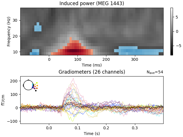
View time-frequency plots#
We now visualize the observed clusters that are statistically significant under our permutation distribution.
Warning
Talking about “significant clusters” can be convenient, but you must be aware of all associated caveats! For example, it is invalid to interpret the cluster p value as being spatially or temporally specific. A cluster with sufficiently low (for example < 0.05) p value at specific location does not allow you to say that the significant effect is at that particular location. The p value only tells you about the probability of obtaining similar or stronger/larger cluster anywhere in the data if there were no differences between the compared conditions. So it only allows you to draw conclusions about the differences in the data “in general”, not at specific locations. See the comprehensive FieldTrip tutorial for more information. FieldTrip tutorial for more information.
evoked_data = evoked.data
times = 1e3 * evoked.times

fig, (ax, ax2) = plt.subplots(2, layout="constrained")

T_obs_plot = np.nan * np.ones_like(T_obs)
for c, p_val in zip(clusters, cluster_p_values):
    if p_val <= 0.05:
        T_obs_plot[c] = T_obs[c]

# Just plot one channel's data
# use the following to show a specific one:
# ch_idx = tfr_epochs.ch_names.index('MEG 1332')
ch_idx, f_idx, t_idx = np.unravel_index(
    np.nanargmax(np.abs(T_obs_plot)), epochs_power.shape[1:]
)

vmax = np.max(np.abs(T_obs))
vmin = -vmax
ax.imshow(
    T_obs[ch_idx],
    cmap=plt.cm.gray,
    extent=[times[0], times[-1], freqs[0], freqs[-1]],
    aspect="auto",
    origin="lower",
    vmin=vmin,
    vmax=vmax,
)
ax.imshow(
    T_obs_plot[ch_idx],
    cmap=plt.cm.RdBu_r,
    extent=[times[0], times[-1], freqs[0], freqs[-1]],
    aspect="auto",
    origin="lower",
    vmin=vmin,
    vmax=vmax,
)
fig.colorbar(ax.images[0])
ax.set(xlabel="Time (ms)", ylabel="Frequency (Hz)")
ax.set(title=f"Induced power ({tfr_epochs.ch_names[ch_idx]})")

evoked.plot(axes=[ax2], time_unit="s")
Total running time of the script: (0 minutes 3.641 seconds)