Plot sensor denoising using oversampled temporal projection#

This demonstrates denoising using the OTP algorithm [1] on data with with sensor artifacts (flux jumps) and random noise.

# Author: Eric Larson <larson.eric.d@gmail.com>
#
# License: BSD-3-Clause
# Copyright the MNE-Python contributors.

import numpy as np

import mne
from mne import find_events, fit_dipole
from mne.datasets.brainstorm import bst_phantom_elekta
from mne.io import read_raw_fif

print(__doc__)

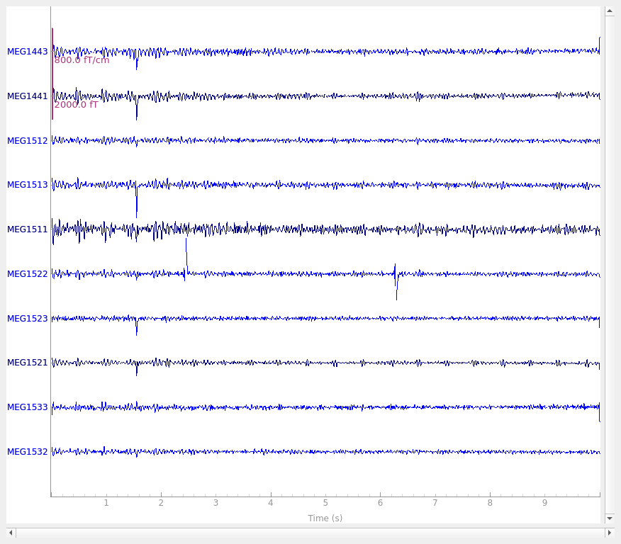
Plot the phantom data, lowpassed to get rid of high-frequency artifacts. We also crop to a single 10-second segment for speed. Notice that there are two large flux jumps on channel 1522 that could spread to other channels when performing subsequent spatial operations (e.g., Maxwell filtering, SSP, or ICA).

dipole_number = 1
data_path = bst_phantom_elekta.data_path()
raw = read_raw_fif(data_path / "kojak_all_200nAm_pp_no_chpi_no_ms_raw.fif")
raw.crop(40.0, 50.0).load_data()
order = list(range(160, 170))
raw.copy().filter(0.0, 40.0).plot(order=order, n_channels=10)

Opening raw data file /home/circleci/mne_data/MNE-brainstorm-data/bst_phantom_elekta/kojak_all_200nAm_pp_no_chpi_no_ms_raw.fif...
    Read a total of 13 projection items:
        planar-0.0-115.0-PCA-01 (1 x 306)  idle
        planar-0.0-115.0-PCA-02 (1 x 306)  idle
        planar-0.0-115.0-PCA-03 (1 x 306)  idle
        planar-0.0-115.0-PCA-04 (1 x 306)  idle
        planar-0.0-115.0-PCA-05 (1 x 306)  idle
        axial-0.0-115.0-PCA-01 (1 x 306)  idle
        axial-0.0-115.0-PCA-02 (1 x 306)  idle
        axial-0.0-115.0-PCA-03 (1 x 306)  idle
        axial-0.0-115.0-PCA-04 (1 x 306)  idle
        axial-0.0-115.0-PCA-05 (1 x 306)  idle
        axial-0.0-115.0-PCA-06 (1 x 306)  idle
        axial-0.0-115.0-PCA-07 (1 x 306)  idle
        axial-0.0-115.0-PCA-08 (1 x 306)  idle
    Range : 47000 ... 437999 =     47.000 ...   437.999 secs
Ready.
Reading 0 ... 10000  =      0.000 ...    10.000 secs...
Filtering raw data in 1 contiguous segment
Setting up low-pass filter at 40 Hz

FIR filter parameters
---------------------
Designing a one-pass, zero-phase, non-causal lowpass filter:
- Windowed time-domain design (firwin) method
- Hamming window with 0.0194 passband ripple and 53 dB stopband attenuation
- Upper passband edge: 40.00 Hz
- Upper transition bandwidth: 10.00 Hz (-6 dB cutoff frequency: 45.00 Hz)
- Filter length: 331 samples (0.331 s)

[Parallel(n_jobs=1)]: Done  17 tasks      | elapsed:    0.0s
[Parallel(n_jobs=1)]: Done  71 tasks      | elapsed:    0.0s
[Parallel(n_jobs=1)]: Done 161 tasks      | elapsed:    0.0s
[Parallel(n_jobs=1)]: Done 287 tasks      | elapsed:    0.1s

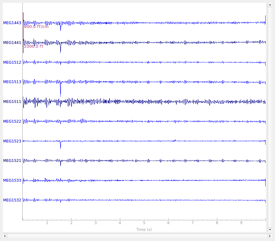
Now we can clean the data with OTP, lowpass, and plot. The flux jumps have been suppressed alongside the random sensor noise.

raw_clean = mne.preprocessing.oversampled_temporal_projection(raw)
raw_clean.filter(0.0, 40.0)
raw_clean.plot(order=order, n_channels=10)

Processing MEG data using oversampled temporal projection
    Processing    1 data chunk of (at least) 10.0 s with 5.0 s overlap and hann windowing
    The final 0.001 s will be lumped into the final window
    Denoising     0.00 –    10.00 s
    Denoising    10.00 –    10.00 s
Filtering raw data in 1 contiguous segment
Setting up low-pass filter at 40 Hz

FIR filter parameters
---------------------
Designing a one-pass, zero-phase, non-causal lowpass filter:
- Windowed time-domain design (firwin) method
- Hamming window with 0.0194 passband ripple and 53 dB stopband attenuation
- Upper passband edge: 40.00 Hz
- Upper transition bandwidth: 10.00 Hz (-6 dB cutoff frequency: 45.00 Hz)
- Filter length: 331 samples (0.331 s)

[Parallel(n_jobs=1)]: Done  17 tasks      | elapsed:    0.0s
[Parallel(n_jobs=1)]: Done  71 tasks      | elapsed:    0.0s
[Parallel(n_jobs=1)]: Done 161 tasks      | elapsed:    0.1s
[Parallel(n_jobs=1)]: Done 287 tasks      | elapsed:    0.1s

We can also look at the effect on single-trial phantom localization. See the Brainstorm Elekta phantom dataset tutorial for more information. Here we use a version that does single-trial localization across the 17 trials are in our 10-second window:

def compute_bias(raw):
    events = find_events(raw, "STI201", verbose=False)
    events = events[1:]  # first one has an artifact
    tmin, tmax = -0.2, 0.1
    epochs = mne.Epochs(
        raw,
        events,
        dipole_number,
        tmin,
        tmax,
        baseline=(None, -0.01),
        preload=True,
        verbose=False,
    )
    sphere = mne.make_sphere_model(r0=(0.0, 0.0, 0.0), head_radius=None, verbose=False)
    cov = mne.compute_covariance(epochs, tmax=0, method="oas", rank=None, verbose=False)
    idx = epochs.time_as_index(0.036)[0]
    data = epochs.get_data(copy=False)[:, :, idx].T
    evoked = mne.EvokedArray(data, epochs.info, tmin=0.0)
    dip = fit_dipole(evoked, cov, sphere, verbose=False)[0]
    actual_pos = mne.dipole.get_phantom_dipoles()[0][dipole_number - 1]
    misses = 1000 * np.linalg.norm(dip.pos - actual_pos, axis=-1)
    return misses


bias = compute_bias(raw)
print(f"Raw bias: {np.mean(bias):0.1f}mm (worst: {np.max(bias):0.1f}mm)")
bias_clean = compute_bias(raw_clean)
print(f"OTP bias: {np.mean(bias_clean):0.1f}mm (worst: {np.max(bias_clean):0.1f}m)")

Raw bias: 2.5mm (worst: 5.2mm)
OTP bias: 1.2mm (worst: 1.4m)

References#

Total running time of the script: (0 minutes 24.090 seconds)

Gallery generated by Sphinx-Gallery