Note
Go to the end to download the full example code.
Compute source level time-frequency timecourses using a DICS beamformer#
In this example, a Dynamic Imaging of Coherent Sources (DICS) [1] beamformer is used to transform sensor-level time-frequency objects to the source level. We will look at the event-related synchronization (ERS) of beta band activity in the somato dataset.
# Authors: Marijn van Vliet <w.m.vanvliet@gmail.com>
#          Alex Rockhill <aprockhill@mailbox.org>
#
# License: BSD-3-Clause
# Copyright the MNE-Python contributors.

import numpy as np

import mne
from mne.beamformer import apply_dics_tfr_epochs, make_dics
from mne.datasets import somato
from mne.time_frequency import csd_tfr

print(__doc__)
Organize the data that we will use for this example.
data_path = somato.data_path()
subject = "01"
task = "somato"
raw_fname = data_path / f"sub-{subject}" / "meg" / f"sub-{subject}_task-{task}_meg.fif"
fname_fwd = (
    data_path / "derivatives" / f"sub-{subject}" / f"sub-{subject}_task-{task}-fwd.fif"
)
subjects_dir = data_path / "derivatives" / "freesurfer" / "subjects"
First, we load the data and compute for each epoch the time-frequency decomposition in sensor space.
# Load raw data and make epochs.
raw = mne.io.read_raw_fif(raw_fname)
events = mne.find_events(raw)
epochs = mne.Epochs(
    raw,
    events[:22],  # just for execution speed of the tutorial
    event_id=1,
    tmin=-1,
    tmax=2.5,
    reject=dict(
        grad=5000e-13,  # unit: T / m (gradiometers)
        mag=5e-12,  # unit: T (magnetometers)
        eog=250e-6,  # unit: V (EOG channels)
    ),
    preload=True,
)

# We are mostly interested in the beta band since it has been shown to be
# active for somatosensory stimulation
freqs = np.linspace(13, 31, 5)

# Use Morlet wavelets to compute sensor-level time-frequency (TFR)
# decomposition for each epoch. We must pass ``output='complex'`` if we wish to
# use this TFR later with a DICS beamformer. We also pass ``average=False`` to
# compute the TFR for each individual epoch.
epochs_tfr = epochs.compute_tfr(
    "morlet", freqs, n_cycles=5, return_itc=False, output="complex", average=False
)

# crop either side to use a buffer to remove edge artifact
epochs_tfr.crop(tmin=-0.5, tmax=2)
Opening raw data file /home/circleci/mne_data/MNE-somato-data/sub-01/meg/sub-01_task-somato_meg.fif...
    Range : 237600 ... 506999 =    791.189 ...  1688.266 secs
Ready.
Finding events on: STI 014
111 events found on stim channel STI 014
Event IDs: [1]
Not setting metadata
22 matching events found
Setting baseline interval to [-0.9989760657919393, 0.0] s
Applying baseline correction (mode: mean)
0 projection items activated
Loading data for 22 events and 1052 original time points ...
    Rejecting  epoch based on MAG : ['MEG 0121']
    Rejecting  epoch based on MAG : ['MEG 0121']
    Rejecting  epoch based on EOG : ['EOG 061']
    Rejecting  epoch based on MAG : ['MEG 0211', 'MEG 1331', 'MEG 2211', 'MEG 2241', 'MEG 2521']
    Rejecting  epoch based on EOG : ['EOG 061']
    Rejecting  epoch based on MAG : ['MEG 1641', 'MEG 1831', 'MEG 1921', 'MEG 1941', 'MEG 2241']
    Rejecting  epoch based on MAG : ['MEG 1831']
    Rejecting  epoch based on MAG : ['MEG 1611']
    Rejecting  epoch based on MAG : ['MEG 0211', 'MEG 0441', 'MEG 1631']
    Rejecting  epoch based on MAG : ['MEG 1611']
    Rejecting  epoch based on MAG : ['MEG 1611', 'MEG 1641']
    Rejecting  epoch based on EOG : ['EOG 061']
12 bad epochs dropped
Now, we build a DICS beamformer and project the sensor-level TFR to the source level.
# Compute the Cross-Spectral Density (CSD) matrix for the sensor-level TFRs.
# We are interested in increases in power relative to the baseline period, so
# we will make a separate CSD for just that period as well.
csd = csd_tfr(epochs_tfr, tmin=-0.5, tmax=2)
baseline_csd = csd_tfr(epochs_tfr, tmin=-0.5, tmax=-0.1)

# use the CSDs and the forward model to build the DICS beamformer
fwd = mne.read_forward_solution(fname_fwd)

# compute scalar DICS beamfomer
filters = make_dics(
    epochs.info,
    fwd,
    csd,
    noise_csd=baseline_csd,
    pick_ori="max-power",
    reduce_rank=True,
    real_filter=True,
)

# project the TFR for each epoch to source space
epochs_stcs = apply_dics_tfr_epochs(epochs_tfr, filters, return_generator=True)

# average across frequencies and epochs
data = np.zeros((fwd["nsource"], epochs_tfr.times.size))
for epoch_stcs in epochs_stcs:
    for stc in epoch_stcs:
        data += (stc.data * np.conj(stc.data)).real

stc.data = data / len(epochs) / len(freqs)

# apply a baseline correction
stc.apply_baseline((-0.5, -0.1))
Reading forward solution from /home/circleci/mne_data/MNE-somato-data/derivatives/sub-01/sub-01_task-somato-fwd.fif...
    Reading a source space...
    [done]
    Reading a source space...
    [done]
    2 source spaces read
    Desired named matrix (kind = 3523 (FIFF_MNE_FORWARD_SOLUTION_GRAD)) not available
    Read MEG forward solution (8155 sources, 306 channels, free orientations)
    Source spaces transformed to the forward solution coordinate frame
Identifying common channels ...
Dropped the following channels:
['STI 014', 'EOG 061', 'STI 001', 'STI 003', 'STI 015', 'STI 004', 'STI 016', 'STI 002', 'STI 006', 'STI 005']
Identifying common channels ...
Computing inverse operator with 306 channels.
    306 out of 306 channels remain after picking
Selected 306 channels
Creating the depth weighting matrix...
Whitening the forward solution.
Computing rank from covariance with rank=None
    Using tolerance 2.8e-14 (2.2e-16 eps * 306 dim * 0.4  max singular value)
    Estimated rank (mag + grad): 64
    MEG: rank 64 computed from 306 data channels with 0 projectors
    Setting small MEG eigenvalues to zero (without PCA)
Creating the source covariance matrix
Adjusting source covariance matrix.
Computing rank from covariance with rank=None
    Using tolerance 2.8e-14 (2.2e-16 eps * 306 dim * 0.4  max singular value)
    Estimated rank (mag + grad): 64
    MEG: rank 64 computed from 306 data channels with 0 projectors
Computing rank from covariance with rank=None
    Using tolerance 8.1e-14 (2.2e-16 eps * 306 dim * 1.2  max singular value)
    Estimated rank (mag + grad): 64
    MEG: rank 64 computed from 306 data channels with 0 projectors
Computing rank from covariance with rank=None
    Using tolerance 3.8e-14 (2.2e-16 eps * 306 dim * 0.56  max singular value)
    Estimated rank (mag + grad): 64
    MEG: rank 64 computed from 306 data channels with 0 projectors
Computing rank from covariance with rank=None
    Using tolerance 1.7e-14 (2.2e-16 eps * 306 dim * 0.26  max singular value)
    Estimated rank (mag + grad): 64
    MEG: rank 64 computed from 306 data channels with 0 projectors
Computing rank from covariance with rank=None
    Using tolerance 9.3e-15 (2.2e-16 eps * 306 dim * 0.14  max singular value)
    Estimated rank (mag + grad): 64
    MEG: rank 64 computed from 306 data channels with 0 projectors
Computing rank from covariance with rank=None
    Using tolerance 5e-15 (2.2e-16 eps * 306 dim * 0.074  max singular value)
    Estimated rank (mag + grad): 64
    MEG: rank 64 computed from 306 data channels with 0 projectors
Computing DICS spatial filters...
    computing DICS spatial filter at 13.0 Hz (1/5)
Computing beamformer filters for 8155 sources
Filter computation complete
    computing DICS spatial filter at 17.5 Hz (2/5)
Computing beamformer filters for 8155 sources
Filter computation complete
    computing DICS spatial filter at 22.0 Hz (3/5)
Computing beamformer filters for 8155 sources
Filter computation complete
    computing DICS spatial filter at 26.5 Hz (4/5)
Computing beamformer filters for 8155 sources
Filter computation complete
    computing DICS spatial filter at 31.0 Hz (5/5)
Computing beamformer filters for 8155 sources
Filter computation complete
Processing epoch : 1
Processing epoch : 2
Processing epoch : 3
Processing epoch : 4
Processing epoch : 5
Processing epoch : 6
Processing epoch : 7
Processing epoch : 8
Processing epoch : 9
Processing epoch : 10
[done]
Applying baseline correction (mode: mean)
Let’s visualize the source time course estimate. We can see the expected activation of the two gyri bordering the central sulcus, the primary somatosensory and motor cortices (S1 and M1).
fmax = 4500
brain = stc.plot(
    subjects_dir=subjects_dir,
    hemi="both",
    views="dorsal",
    initial_time=1.2,
    brain_kwargs=dict(show=False),
    add_data_kwargs=dict(
        fmin=fmax / 10,
        fmid=fmax / 2,
        fmax=fmax,
        scale_factor=0.0001,
        colorbar_kwargs=dict(label_font_size=10),
    ),
)
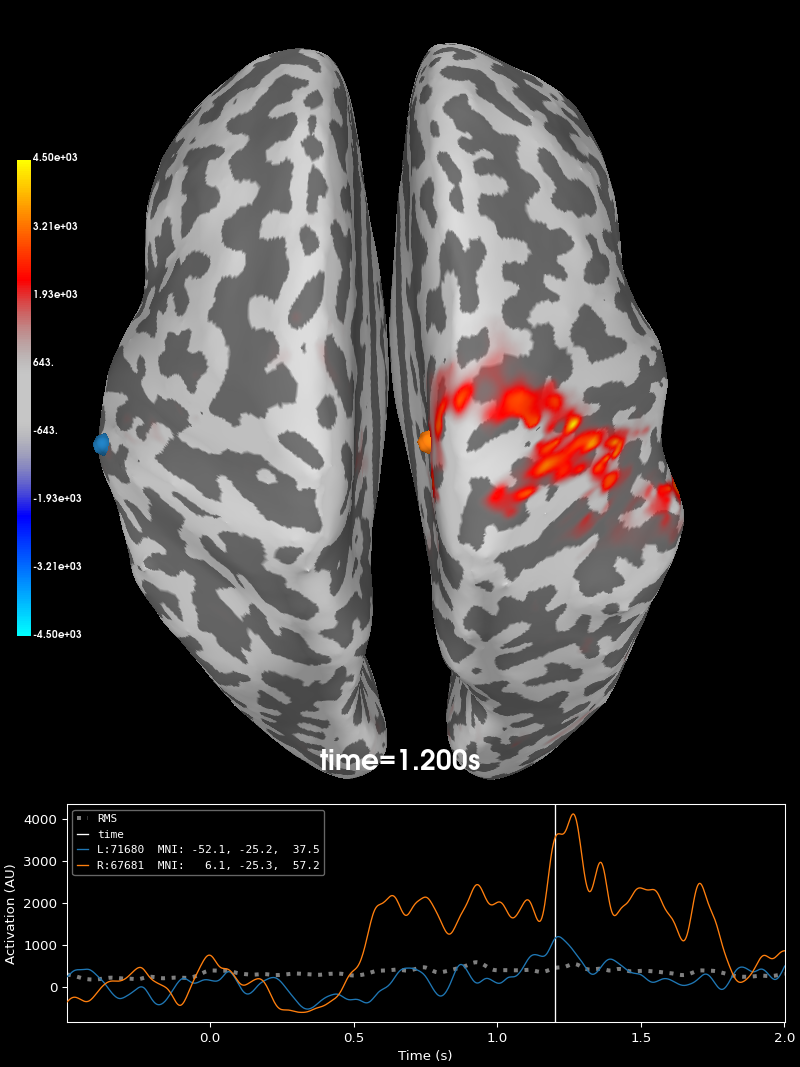
Using control points [ 688.33913449 817.80202112 3163.68479992]
Total running time of the script: (0 minutes 53.059 seconds)