Note
Go to the end to download the full example code.
Compute spatial resolution metrics in source space#
Compute peak localisation error and spatial deviation for the point-spread functions of dSPM and MNE. Plot their distributions and difference of distributions. This example mimics some results from [1], namely Figure 3 (peak localisation error for PSFs, L2-MNE vs dSPM) and Figure 4 (spatial deviation for PSFs, L2-MNE vs dSPM).
# Author: Olaf Hauk <olaf.hauk@mrc-cbu.cam.ac.uk>
#
# License: BSD-3-Clause
# Copyright the MNE-Python contributors.
import mne
from mne.datasets import sample
from mne.minimum_norm import make_inverse_resolution_matrix, resolution_metrics

print(__doc__)

data_path = sample.data_path()
subjects_dir = data_path / "subjects"
meg_path = data_path / "MEG" / "sample"
fname_fwd = meg_path / "sample_audvis-meg-eeg-oct-6-fwd.fif"
fname_cov = meg_path / "sample_audvis-cov.fif"
fname_evo = meg_path / "sample_audvis-ave.fif"

# read forward solution
forward = mne.read_forward_solution(fname_fwd)
# forward operator with fixed source orientations
mne.convert_forward_solution(forward, surf_ori=True, force_fixed=True, copy=False)

# noise covariance matrix
noise_cov = mne.read_cov(fname_cov)

# evoked data for info
evoked = mne.read_evokeds(fname_evo, 0)

# make inverse operator from forward solution
# free source orientation
inverse_operator = mne.minimum_norm.make_inverse_operator(
    info=evoked.info, forward=forward, noise_cov=noise_cov, loose=0.0, depth=None
)

# regularisation parameter
snr = 3.0
lambda2 = 1.0 / snr**2
Reading forward solution from /home/circleci/mne_data/MNE-sample-data/MEG/sample/sample_audvis-meg-eeg-oct-6-fwd.fif...
    Reading a source space...
    Computing patch statistics...
    Patch information added...
    Distance information added...
    [done]
    Reading a source space...
    Computing patch statistics...
    Patch information added...
    Distance information added...
    [done]
    2 source spaces read
    Desired named matrix (kind = 3523 (FIFF_MNE_FORWARD_SOLUTION_GRAD)) not available
    Read MEG forward solution (7498 sources, 306 channels, free orientations)
    Desired named matrix (kind = 3523 (FIFF_MNE_FORWARD_SOLUTION_GRAD)) not available
    Read EEG forward solution (7498 sources, 60 channels, free orientations)
    Forward solutions combined: MEG, EEG
    Source spaces transformed to the forward solution coordinate frame
    Average patch normals will be employed in the rotation to the local surface coordinates....
    Converting to surface-based source orientations...
    [done]
    366 x 366 full covariance (kind = 1) found.
    Read a total of 4 projection items:
        PCA-v1 (1 x 10²) active
        PCA-v2 (1 x 10²) active
        PCA-v3 (1 x 10²) active
        Average EEG reference (1 x 60) active
Reading /home/circleci/mne_data/MNE-sample-data/MEG/sample/sample_audvis-ave.fif ...
    Read a total of 4 projection items:
        PCA-v1 (1 x 10²) active
        PCA-v2 (1 x 10²) active
        PCA-v3 (1 x 10²) active
        Average EEG reference (1 x 60) active
    Found the data of interest:
        t =    -199.80 ...     499.49 ms (Left Auditory)
        0 CTF compensation matrices available
        nave = 55 - aspect type = 100
Projections have already been applied. Setting proj attribute to True.
No baseline correction applied
Computing inverse operator with 364 channels.
    364 out of 366 channels remain after picking
Selected 364 channels
Whitening the forward solution.
    Created an SSP operator (subspace dimension = 4)
Computing rank from covariance with rank=None
    Using tolerance 3.3e-13 (2.2e-16 eps * 305 dim * 4.8  max singular value)
    Estimated rank (mag + grad): 302
    MEG: rank 302 computed from 305 data channels with 3 projectors
    Using tolerance 4.7e-14 (2.2e-16 eps * 59 dim * 3.6  max singular value)
    Estimated rank (eeg): 58
    EEG: rank 58 computed from 59 data channels with 1 projector
    Setting small MEG eigenvalues to zero (without PCA)
    Setting small EEG eigenvalues to zero (without PCA)
Creating the source covariance matrix
Adjusting source covariance matrix.
Computing SVD of whitened and weighted lead field matrix.
    largest singular value = 4.31738
    scaling factor to adjust the trace = 1.68644e+20 (nchan = 364 nzero = 4)
MNE#
Compute resolution matrices, peak localisation error (PLE) for point spread functions (PSFs), spatial deviation (SD) for PSFs:
rm_mne = make_inverse_resolution_matrix(
    forward, inverse_operator, method="MNE", lambda2=lambda2
)
ple_mne_psf = resolution_metrics(
    rm_mne, inverse_operator["src"], function="psf", metric="peak_err"
)
sd_mne_psf = resolution_metrics(
    rm_mne, inverse_operator["src"], function="psf", metric="sd_ext"
)
del rm_mne
    364 out of 366 channels remain after picking
Preparing the inverse operator for use...
    Scaled noise and source covariance from nave = 1 to nave = 1
    Created the regularized inverter
    Created an SSP operator (subspace dimension = 4)
    Created the whitener using a noise covariance matrix with rank 360 (4 small eigenvalues omitted)
Applying inverse operator to ""...
    Picked 364 channels from the data
    Computing inverse...
    Eigenleads need to be weighted ...
    Computing residual...
    Explained  43.2% variance
[done]
Dimension of Inverse Matrix: (7498, 364)
Dimensions of resolution matrix: 7498 by 7498.
dSPM#
Do the same for dSPM:
rm_dspm = make_inverse_resolution_matrix(
    forward, inverse_operator, method="dSPM", lambda2=lambda2
)
ple_dspm_psf = resolution_metrics(
    rm_dspm, inverse_operator["src"], function="psf", metric="peak_err"
)
sd_dspm_psf = resolution_metrics(
    rm_dspm, inverse_operator["src"], function="psf", metric="sd_ext"
)
del rm_dspm, forward
    364 out of 366 channels remain after picking
Preparing the inverse operator for use...
    Scaled noise and source covariance from nave = 1 to nave = 1
    Created the regularized inverter
    Created an SSP operator (subspace dimension = 4)
    Created the whitener using a noise covariance matrix with rank 360 (4 small eigenvalues omitted)
    Computing noise-normalization factors (dSPM)...
[done]
Applying inverse operator to ""...
    Picked 364 channels from the data
    Computing inverse...
    Eigenleads need to be weighted ...
    Computing residual...
    Explained  43.2% variance
    dSPM...
[done]
Dimension of Inverse Matrix: (7498, 364)
Dimensions of resolution matrix: 7498 by 7498.
Visualize results#
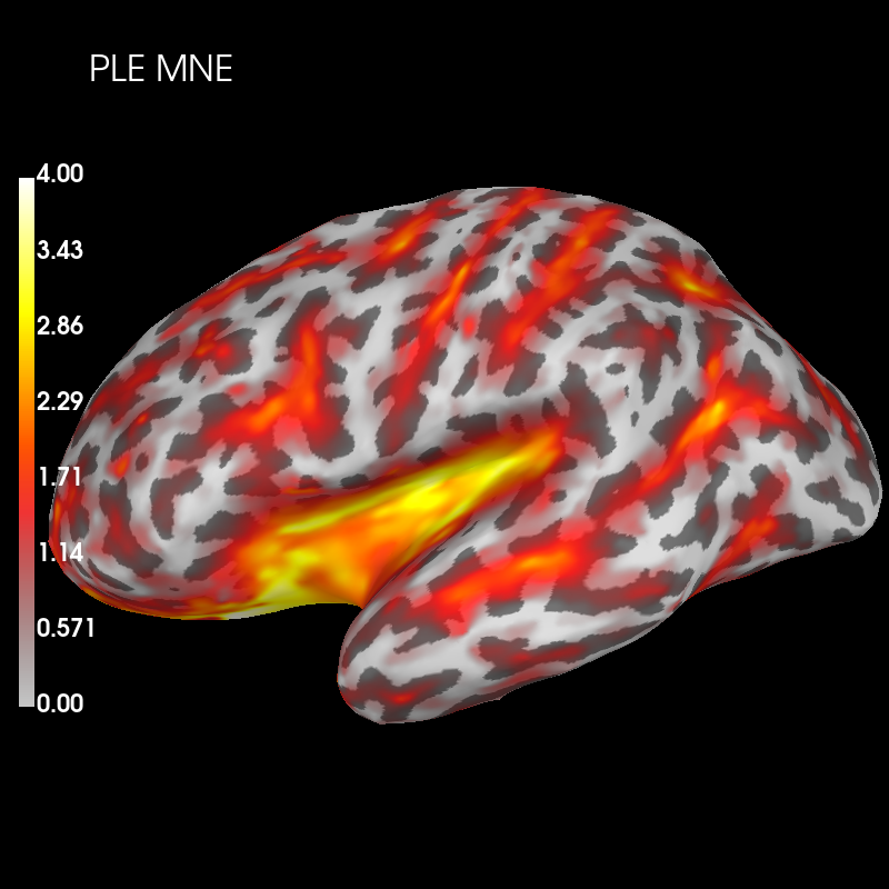
Visualise peak localisation error (PLE) across the whole cortex for MNE PSF:
brain_ple_mne = ple_mne_psf.plot(
    "sample",
    "inflated",
    "lh",
    subjects_dir=subjects_dir,
    figure=1,
    clim=dict(kind="value", lims=(0, 2, 4)),
)
brain_ple_mne.add_text(0.1, 0.9, "PLE MNE", "title", font_size=16)
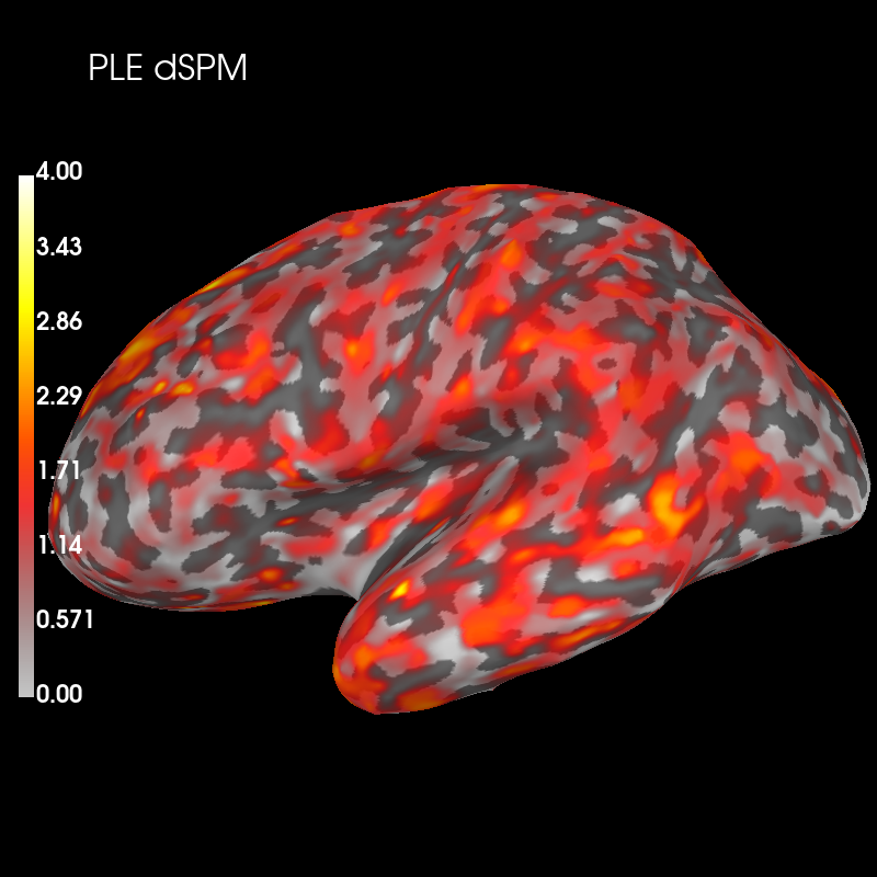
And dSPM:
brain_ple_dspm = ple_dspm_psf.plot(
    "sample",
    "inflated",
    "lh",
    subjects_dir=subjects_dir,
    figure=2,
    clim=dict(kind="value", lims=(0, 2, 4)),
)
brain_ple_dspm.add_text(0.1, 0.9, "PLE dSPM", "title", font_size=16)
Subtract the two distributions and plot this difference
diff_ple = ple_mne_psf - ple_dspm_psf

brain_ple_diff = diff_ple.plot(
    "sample",
    "inflated",
    "lh",
    subjects_dir=subjects_dir,
    figure=3,
    clim=dict(kind="value", pos_lims=(0.0, 1.0, 2.0)),
)
brain_ple_diff.add_text(0.1, 0.9, "PLE MNE-dSPM", "title", font_size=16)
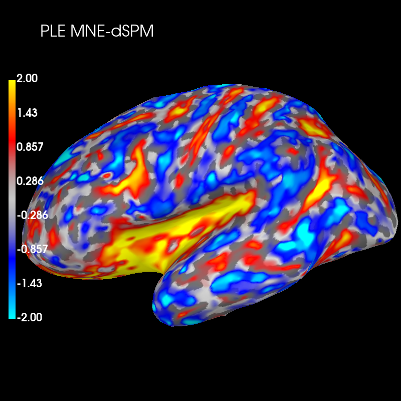
These plots show that dSPM has generally lower peak localization error (red color) than MNE in deeper brain areas, but higher error (blue color) in more superficial areas.
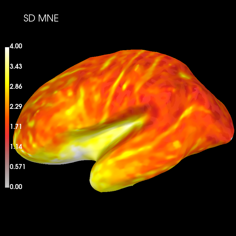
Next we’ll visualise spatial deviation (SD) across the whole cortex for MNE PSF:
brain_sd_mne = sd_mne_psf.plot(
    "sample",
    "inflated",
    "lh",
    subjects_dir=subjects_dir,
    figure=4,
    clim=dict(kind="value", lims=(0, 2, 4)),
)
brain_sd_mne.add_text(0.1, 0.9, "SD MNE", "title", font_size=16)
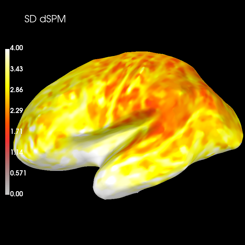
And dSPM:
brain_sd_dspm = sd_dspm_psf.plot(
    "sample",
    "inflated",
    "lh",
    subjects_dir=subjects_dir,
    figure=5,
    clim=dict(kind="value", lims=(0, 2, 4)),
)
brain_sd_dspm.add_text(0.1, 0.9, "SD dSPM", "title", font_size=16)
Subtract the two distributions and plot this difference:
diff_sd = sd_mne_psf - sd_dspm_psf

brain_sd_diff = diff_sd.plot(
    "sample",
    "inflated",
    "lh",
    subjects_dir=subjects_dir,
    figure=6,
    clim=dict(kind="value", pos_lims=(0.0, 1.0, 2.0)),
)
brain_sd_diff.add_text(0.1, 0.9, "SD MNE-dSPM", "title", font_size=16)
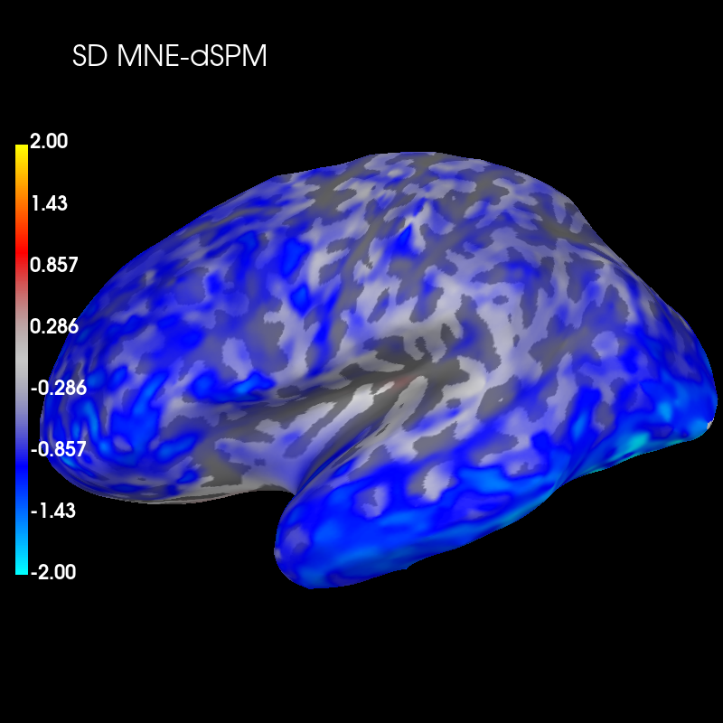
These plots show that dSPM has generally higher spatial deviation than MNE (blue color), i.e. worse performance to distinguish different sources.
References#
Total running time of the script: (0 minutes 31.670 seconds)