Getting impedances from raw files

Many EEG systems provide impedance measurements for each channel within their file format. MNE does not parse this information and does not store it in the Raw object. However, it is possible to extract this information from the raw data and store it in a separate data structure.

ANT Neuro

The .cnt file format from ANT Neuro stores impedance information in the form of triggers. The function mne.io.read_raw_ant() reads this information and marks the time-segment during which an impedance measurement was performed as Annotations with the description set in the argument impedance_annotation. However, it doesn’t extract the impedance values themselves. To do so, use the function antio.parser.read_triggers.

# Authors: The MNE-Python contributors.
# License: BSD-3-Clause
# Copyright the MNE-Python contributors.

import numpy as np
from antio import read_cnt
from antio.parser import read_triggers
from matplotlib import pyplot as plt
from mffpy.xml_files import DataInfo

from mne.datasets import testing
from mne.io import read_raw_ant, read_raw_egi
from mne.viz import plot_topomap

fname = testing.data_path() / "antio" / "CA_208" / "test_CA_208.cnt"
cnt = read_cnt(fname)
_, _, _, impedances, _ = read_triggers(cnt)

raw = read_raw_ant(fname, eog=r"EOG")
impedances = [{ch: imp[k] for k, ch in enumerate(raw.ch_names)} for imp in impedances]
print(impedances[0])  # impedances measurement at the beginning of the recording

Reading ANT file /home/circleci/mne_data/MNE-testing-data/antio/CA_208/test_CA_208.cnt
All 63 EEG channels are referenced to CPz.
{'Fp1': 2.254, 'Fpz': 2.926, 'Fp2': 2.693, 'F7': 13.045, 'F3': 0.902, 'Fz': 2.737, 'F4': 0.149, 'F8': 25.132999, 'FC5': 0.304, 'FC1': 38.924, 'FC2': 2.258, 'FC6': 0.135, 'M1': 4.445, 'T7': 6.233, 'C3': 8.322, 'Cz': 0.064, 'C4': 1.271, 'T8': 4.049, 'M2': 1.846, 'CP5': 2.721, 'CP1': 2.944, 'CP2': 1.218, 'CP6': 0.879, 'P7': 22.726999, 'P3': 9.176, 'Pz': 1.84, 'P4': 27.167, 'P8': 1.157, 'POz': 3.575, 'O1': 2.698, 'O2': 8.073, 'EOG': 15.205, 'AF7': 5.842, 'AF3': 1.303, 'AF4': 2.136, 'AF8': 0.787, 'F5': 0.863, 'F1': 1.696, 'F2': 1.616, 'F6': 0.478, 'FC3': 6.01, 'FCz': 0.72, 'FC4': 4.314, 'C5': 10.945, 'C1': 6.151, 'C2': 0.772, 'C6': 0.879, 'CP3': 12.115, 'CP4': 1.887, 'P5': 14.045, 'P1': 2.733, 'P2': 34.641998, 'P6': 1.765, 'PO5': 5.666, 'PO3': 14.12, 'PO4': 2.599, 'PO6': 11.339, 'FT7': 13.158, 'FT8': 1.046, 'TP7': 5.917, 'TP8': 2.61, 'PO7': 5.691, 'PO8': 1.759, 'Oz': 5.165, 'BIP1': 2147483.75, 'BIP2': 2147483.75, 'BIP3': 2147483.75, 'BIP4': 2147483.75, 'BIP5': 2147483.75, 'BIP6': 2147483.75, 'BIP7': 2147483.75, 'BIP8': 2147483.75, 'BIP9': 2147483.75, 'BIP10': 2147483.75, 'BIP11': 2147483.75, 'BIP12': 2147483.75, 'BIP13': 2147483.75, 'BIP14': 2147483.75, 'BIP15': 2147483.75, 'BIP16': 2147483.75, 'BIP17': 2147483.75, 'BIP18': 2147483.75, 'BIP19': 2147483.75, 'BIP20': 2147483.75, 'BIP21': 2147483.75, 'BIP22': 2147483.75, 'BIP23': 2147483.75, 'BIP24': 2147483.75}

Note that the impedance measurement contains all channels, including the bipolar ones. We can visualize the impedances on a topographic map; below we show a topography of impedances before and after the recording for the EEG channels only.

raw.pick("eeg").set_montage("colin27_1020")
impedances = [{ch: imp[ch] for ch in raw.ch_names} for imp in impedances]

f, ax = plt.subplots(1, 2, layout="constrained", figsize=(10, 5))
f.suptitle("Impedances (kOhm)")
impedance = list(impedances[0].values())
plot_topomap(
    impedance,
    raw.info,
    vlim=(0, 50),
    axes=ax[0],
    show=False,
    names=[f"{elt:.1f}" for elt in impedance],
)
ax[0].set_title("Impedances at the beginning of the recording")
impedance = list(impedances[-1].values())
plot_topomap(
    impedance,
    raw.info,
    vlim=(0, 50),
    axes=ax[1],
    show=False,
    names=[f"{elt:.1f}" for elt in impedance],
)
ax[1].set_title("Impedances at the end of the recording")
plt.show()

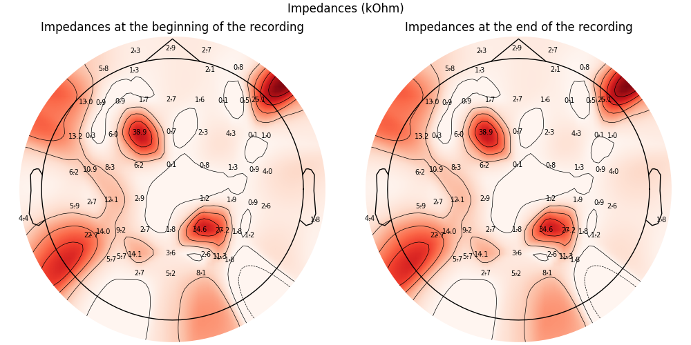
In this very short test file, the impedances are stable over time.

EGI

EGI MFF files store per-channel gain (GCAL) and impedance (ICAL) calibration data in info1.xml inside the .mff directory. mne.io.read_raw_egi() does not expose this information in the Raw object, but it can be read directly from info1.xml via mffpy.

Open the MFF file, keep only EEG channels, then read the calibration block from info1.xml. The ICAL entry holds one impedance value per channel (in kΩ) at the time calibration was performed; GCAL holds per-channel gain correction factors (close to 1.0).

fname_egi = testing.data_path() / "EGI" / "test_egi.mff"
raw_egi = read_raw_egi(fname_egi, verbose=False)
raw_egi.pick("eeg")

data_info = DataInfo.from_file(fname_egi / "info1.xml")
ical = data_info.calibrations["ICAL"]["channels"]  # 1-indexed dict, values in kΩ

# Channel order in raw matches the 1-indexed calibration keys.
ical_vals = np.array([ical.get(i + 1, np.nan) for i in range(len(raw_egi.ch_names))])
print({ch: round(float(v), 1) for ch, v in zip(raw_egi.ch_names[:5], ical_vals[:5])})

{'E1': 19.8, 'E2': 21.6, 'E3': 18.9, 'E4': 25.3, 'E5': 29.2}

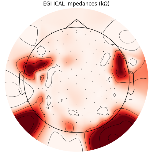
Visualize the per-channel ICAL impedances on a topographic map.

fig, ax = plt.subplots(layout="constrained", figsize=(5, 5))
plot_topomap(ical_vals, raw_egi.info, axes=ax, show=False)
ax.set_title("EGI ICAL impedances (kΩ)")
plt.show()