Note
Go to the end to download the full example code.
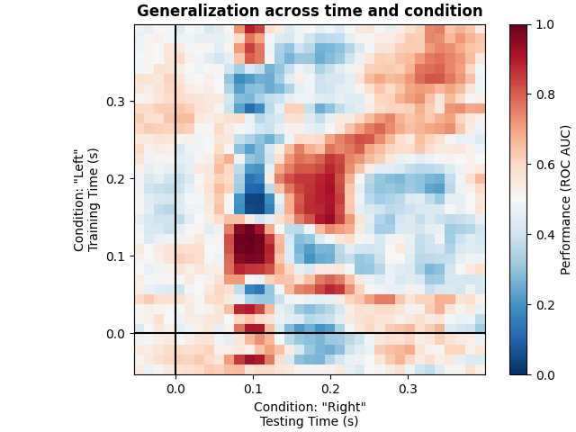
Decoding sensor space data with generalization across time and conditions#
This example runs the analysis described in [1]. It illustrates how one can fit a linear classifier to identify a discriminatory topography at a given time instant and subsequently assess whether this linear model can accurately predict all of the time samples of a second set of conditions.
# Authors: Jean-Remi King <jeanremi.king@gmail.com>
# Alexandre Gramfort <alexandre.gramfort@inria.fr>
# Denis Engemann <denis.engemann@gmail.com>
#
# License: BSD-3-Clause
# Copyright the MNE-Python contributors.
import matplotlib.pyplot as plt
from sklearn.linear_model import LogisticRegression
from sklearn.pipeline import make_pipeline
from sklearn.preprocessing import StandardScaler
import mne
from mne.datasets import sample
from mne.decoding import GeneralizingEstimator
print(__doc__)
# Preprocess data
data_path = sample.data_path()
# Load and filter data, set up epochs
meg_path = data_path / "MEG" / "sample"
raw_fname = meg_path / "sample_audvis_filt-0-40_raw.fif"
events_fname = meg_path / "sample_audvis_filt-0-40_raw-eve.fif"
raw = mne.io.read_raw_fif(raw_fname, preload=True)
picks = mne.pick_types(raw.info, meg=True, exclude="bads") # Pick MEG channels
raw.filter(1.0, 30.0, fir_design="firwin") # Band pass filtering signals
events = mne.read_events(events_fname)
event_id = {
"Auditory/Left": 1,
"Auditory/Right": 2,
"Visual/Left": 3,
"Visual/Right": 4,
}
tmin = -0.050
tmax = 0.400
# decimate to make the example faster to run, but then use verbose='error' in
# the Epochs constructor to suppress warning about decimation causing aliasing
decim = 2
epochs = mne.Epochs(
raw,
events,
event_id=event_id,
tmin=tmin,
tmax=tmax,
proj=True,
picks=picks,
baseline=None,
preload=True,
reject=dict(mag=5e-12),
decim=decim,
verbose="error",
)
Opening raw data file /home/circleci/mne_data/MNE-sample-data/MEG/sample/sample_audvis_filt-0-40_raw.fif...
Read a total of 4 projection items:
PCA-v1 (1 x 10²) idle
PCA-v2 (1 x 10²) idle
PCA-v3 (1 x 10²) idle
Average EEG reference (1 x 60) idle
Range : 6450 ... 48149 = 42.956 ... 320.665 secs
Ready.
Reading 0 ... 41699 = 0.000 ... 277.709 secs...
Filtering raw data in 1 contiguous segment
Setting up band-pass filter from 1 - 30 Hz
FIR filter parameters
---------------------
Designing a one-pass, zero-phase, non-causal bandpass filter:
- Windowed time-domain design (firwin) method
- Hamming window with 0.0194 passband ripple and 53 dB stopband attenuation
- Lower passband edge: 1.00
- Lower transition bandwidth: 1.00 Hz (-6 dB cutoff frequency: 0.50 Hz)
- Upper passband edge: 30.00 Hz
- Upper transition bandwidth: 7.50 Hz (-6 dB cutoff frequency: 33.75 Hz)
- Filter length: 497 samples (3.310 s)
[Parallel(n_jobs=1)]: Done 17 tasks | elapsed: 0.0s
[Parallel(n_jobs=1)]: Done 71 tasks | elapsed: 0.1s
[Parallel(n_jobs=1)]: Done 161 tasks | elapsed: 0.3s
[Parallel(n_jobs=1)]: Done 287 tasks | elapsed: 0.5s
We will train the classifier on all left visual vs auditory trials and test on all right visual vs auditory trials.
clf = make_pipeline(
StandardScaler(),
LogisticRegression(solver="liblinear"), # liblinear is faster than lbfgs
)
time_gen = GeneralizingEstimator(clf, scoring="roc_auc", n_jobs=None, verbose=True)
# Fit classifiers on the epochs where the stimulus was presented to the left.
# Note that the experimental condition y indicates auditory or visual
time_gen.fit(X=epochs["Left"].get_data(copy=False), y=epochs["Left"].events[:, 2] > 2)
0%| | Fitting GeneralizingEstimator : 0/35 [00:00<?, ?it/s]
3%|▎ | Fitting GeneralizingEstimator : 1/35 [00:00<00:01, 29.12it/s]
9%|▊ | Fitting GeneralizingEstimator : 3/35 [00:00<00:00, 44.30it/s]
14%|█▍ | Fitting GeneralizingEstimator : 5/35 [00:00<00:00, 49.10it/s]
17%|█▋ | Fitting GeneralizingEstimator : 6/35 [00:00<00:00, 43.90it/s]
23%|██▎ | Fitting GeneralizingEstimator : 8/35 [00:00<00:00, 47.24it/s]
31%|███▏ | Fitting GeneralizingEstimator : 11/35 [00:00<00:00, 54.98it/s]
40%|████ | Fitting GeneralizingEstimator : 14/35 [00:00<00:00, 60.51it/s]
49%|████▊ | Fitting GeneralizingEstimator : 17/35 [00:00<00:00, 64.64it/s]
57%|█████▋ | Fitting GeneralizingEstimator : 20/35 [00:00<00:00, 67.85it/s]
63%|██████▎ | Fitting GeneralizingEstimator : 22/35 [00:00<00:00, 66.75it/s]
71%|███████▏ | Fitting GeneralizingEstimator : 25/35 [00:00<00:00, 69.03it/s]
74%|███████▍ | Fitting GeneralizingEstimator : 26/35 [00:00<00:00, 64.78it/s]
83%|████████▎ | Fitting GeneralizingEstimator : 29/35 [00:00<00:00, 67.23it/s]
89%|████████▊ | Fitting GeneralizingEstimator : 31/35 [00:00<00:00, 66.45it/s]
97%|█████████▋| Fitting GeneralizingEstimator : 34/35 [00:00<00:00, 68.53it/s]
100%|██████████| Fitting GeneralizingEstimator : 35/35 [00:00<00:00, 67.50it/s]
Score on the epochs where the stimulus was presented to the right.
scores = time_gen.score(
X=epochs["Right"].get_data(copy=False), y=epochs["Right"].events[:, 2] > 2
)
0%| | Scoring GeneralizingEstimator : 0/1225 [00:00<?, ?it/s]
1%| | Scoring GeneralizingEstimator : 10/1225 [00:00<00:04, 292.15it/s]
2%|▏ | Scoring GeneralizingEstimator : 23/1225 [00:00<00:03, 336.46it/s]
3%|▎ | Scoring GeneralizingEstimator : 34/1225 [00:00<00:03, 331.38it/s]
4%|▍ | Scoring GeneralizingEstimator : 48/1225 [00:00<00:03, 353.42it/s]
5%|▍ | Scoring GeneralizingEstimator : 61/1225 [00:00<00:03, 359.19it/s]
6%|▌ | Scoring GeneralizingEstimator : 74/1225 [00:00<00:03, 363.60it/s]
7%|▋ | Scoring GeneralizingEstimator : 88/1225 [00:00<00:03, 371.75it/s]
8%|▊ | Scoring GeneralizingEstimator : 103/1225 [00:00<00:02, 382.37it/s]
10%|▉ | Scoring GeneralizingEstimator : 117/1225 [00:00<00:02, 385.80it/s]
11%|█ | Scoring GeneralizingEstimator : 132/1225 [00:00<00:02, 392.27it/s]
12%|█▏ | Scoring GeneralizingEstimator : 147/1225 [00:00<00:02, 398.13it/s]
13%|█▎ | Scoring GeneralizingEstimator : 162/1225 [00:00<00:02, 403.12it/s]
14%|█▍ | Scoring GeneralizingEstimator : 177/1225 [00:00<00:02, 406.84it/s]
15%|█▌ | Scoring GeneralizingEstimator : 189/1225 [00:00<00:02, 401.65it/s]
17%|█▋ | Scoring GeneralizingEstimator : 203/1225 [00:00<00:02, 402.71it/s]
18%|█▊ | Scoring GeneralizingEstimator : 217/1225 [00:00<00:02, 403.62it/s]
19%|█▉ | Scoring GeneralizingEstimator : 231/1225 [00:00<00:02, 404.29it/s]
20%|██ | Scoring GeneralizingEstimator : 246/1225 [00:00<00:02, 406.85it/s]
21%|██▏ | Scoring GeneralizingEstimator : 261/1225 [00:00<00:02, 409.54it/s]
23%|██▎ | Scoring GeneralizingEstimator : 276/1225 [00:00<00:02, 412.27it/s]
24%|██▍ | Scoring GeneralizingEstimator : 291/1225 [00:00<00:02, 414.70it/s]
25%|██▌ | Scoring GeneralizingEstimator : 307/1225 [00:00<00:02, 419.02it/s]
26%|██▋ | Scoring GeneralizingEstimator : 322/1225 [00:00<00:02, 420.44it/s]
28%|██▊ | Scoring GeneralizingEstimator : 337/1225 [00:00<00:02, 422.07it/s]
29%|██▉ | Scoring GeneralizingEstimator : 353/1225 [00:00<00:02, 425.63it/s]
30%|███ | Scoring GeneralizingEstimator : 368/1225 [00:00<00:02, 426.84it/s]
31%|███▏ | Scoring GeneralizingEstimator : 384/1225 [00:00<00:01, 429.76it/s]
33%|███▎ | Scoring GeneralizingEstimator : 399/1225 [00:00<00:01, 430.21it/s]
34%|███▍ | Scoring GeneralizingEstimator : 414/1225 [00:00<00:01, 431.07it/s]
35%|███▍ | Scoring GeneralizingEstimator : 428/1225 [00:01<00:01, 430.03it/s]
36%|███▌ | Scoring GeneralizingEstimator : 443/1225 [00:01<00:01, 430.88it/s]
37%|███▋ | Scoring GeneralizingEstimator : 456/1225 [00:01<00:01, 427.73it/s]
38%|███▊ | Scoring GeneralizingEstimator : 470/1225 [00:01<00:01, 426.88it/s]
39%|███▉ | Scoring GeneralizingEstimator : 480/1225 [00:01<00:01, 418.88it/s]
40%|████ | Scoring GeneralizingEstimator : 494/1225 [00:01<00:01, 418.25it/s]
41%|████▏ | Scoring GeneralizingEstimator : 508/1225 [00:01<00:01, 417.62it/s]
43%|████▎ | Scoring GeneralizingEstimator : 524/1225 [00:01<00:01, 420.84it/s]
44%|████▍ | Scoring GeneralizingEstimator : 539/1225 [00:01<00:01, 422.14it/s]
45%|████▌ | Scoring GeneralizingEstimator : 553/1225 [00:01<00:01, 421.67it/s]
46%|████▌ | Scoring GeneralizingEstimator : 564/1225 [00:01<00:01, 415.89it/s]
47%|████▋ | Scoring GeneralizingEstimator : 577/1225 [00:01<00:01, 413.81it/s]
48%|████▊ | Scoring GeneralizingEstimator : 588/1225 [00:01<00:01, 408.89it/s]
49%|████▉ | Scoring GeneralizingEstimator : 602/1225 [00:01<00:01, 409.12it/s]
50%|█████ | Scoring GeneralizingEstimator : 618/1225 [00:01<00:01, 412.74it/s]
52%|█████▏ | Scoring GeneralizingEstimator : 632/1225 [00:01<00:01, 412.85it/s]
53%|█████▎ | Scoring GeneralizingEstimator : 646/1225 [00:01<00:01, 412.97it/s]
54%|█████▍ | Scoring GeneralizingEstimator : 660/1225 [00:01<00:01, 412.78it/s]
55%|█████▌ | Scoring GeneralizingEstimator : 676/1225 [00:01<00:01, 415.78it/s]
56%|█████▋ | Scoring GeneralizingEstimator : 691/1225 [00:01<00:01, 416.89it/s]
57%|█████▋ | Scoring GeneralizingEstimator : 701/1225 [00:01<00:01, 410.23it/s]
58%|█████▊ | Scoring GeneralizingEstimator : 712/1225 [00:01<00:01, 405.32it/s]
59%|█████▉ | Scoring GeneralizingEstimator : 720/1225 [00:01<00:01, 396.31it/s]
60%|█████▉ | Scoring GeneralizingEstimator : 731/1225 [00:01<00:01, 392.55it/s]
61%|██████ | Scoring GeneralizingEstimator : 745/1225 [00:01<00:01, 393.57it/s]
62%|██████▏ | Scoring GeneralizingEstimator : 759/1225 [00:01<00:01, 394.63it/s]
63%|██████▎ | Scoring GeneralizingEstimator : 772/1225 [00:01<00:01, 394.04it/s]
64%|██████▍ | Scoring GeneralizingEstimator : 783/1225 [00:01<00:01, 390.42it/s]
65%|██████▍ | Scoring GeneralizingEstimator : 796/1225 [00:01<00:01, 390.13it/s]
66%|██████▌ | Scoring GeneralizingEstimator : 811/1225 [00:02<00:01, 392.87it/s]
67%|██████▋ | Scoring GeneralizingEstimator : 825/1225 [00:02<00:01, 393.94it/s]
68%|██████▊ | Scoring GeneralizingEstimator : 838/1225 [00:02<00:00, 393.48it/s]
70%|██████▉ | Scoring GeneralizingEstimator : 853/1225 [00:02<00:00, 396.10it/s]
71%|███████ | Scoring GeneralizingEstimator : 869/1225 [00:02<00:00, 399.94it/s]
72%|███████▏ | Scoring GeneralizingEstimator : 885/1225 [00:02<00:00, 403.57it/s]
73%|███████▎ | Scoring GeneralizingEstimator : 899/1225 [00:02<00:00, 404.04it/s]
75%|███████▍ | Scoring GeneralizingEstimator : 915/1225 [00:02<00:00, 407.64it/s]
76%|███████▌ | Scoring GeneralizingEstimator : 930/1225 [00:02<00:00, 409.53it/s]
77%|███████▋ | Scoring GeneralizingEstimator : 946/1225 [00:02<00:00, 412.54it/s]
78%|███████▊ | Scoring GeneralizingEstimator : 960/1225 [00:02<00:00, 412.66it/s]
80%|███████▉ | Scoring GeneralizingEstimator : 975/1225 [00:02<00:00, 414.26it/s]
81%|████████ | Scoring GeneralizingEstimator : 989/1225 [00:02<00:00, 414.03it/s]
82%|████████▏ | Scoring GeneralizingEstimator : 1005/1225 [00:02<00:00, 417.04it/s]
83%|████████▎ | Scoring GeneralizingEstimator : 1012/1225 [00:02<00:00, 406.35it/s]
84%|████████▎ | Scoring GeneralizingEstimator : 1024/1225 [00:02<00:00, 403.24it/s]
85%|████████▍ | Scoring GeneralizingEstimator : 1037/1225 [00:02<00:00, 402.32it/s]
86%|████████▌ | Scoring GeneralizingEstimator : 1052/1225 [00:02<00:00, 404.20it/s]
87%|████████▋ | Scoring GeneralizingEstimator : 1067/1225 [00:02<00:00, 406.18it/s]
88%|████████▊ | Scoring GeneralizingEstimator : 1083/1225 [00:02<00:00, 409.41it/s]
90%|████████▉ | Scoring GeneralizingEstimator : 1098/1225 [00:02<00:00, 411.02it/s]
91%|█████████ | Scoring GeneralizingEstimator : 1114/1225 [00:02<00:00, 413.89it/s]
92%|█████████▏| Scoring GeneralizingEstimator : 1130/1225 [00:02<00:00, 416.88it/s]
93%|█████████▎| Scoring GeneralizingEstimator : 1140/1225 [00:02<00:00, 410.74it/s]
94%|█████████▍| Scoring GeneralizingEstimator : 1150/1225 [00:02<00:00, 404.98it/s]
95%|█████████▍| Scoring GeneralizingEstimator : 1161/1225 [00:02<00:00, 400.95it/s]
96%|█████████▌| Scoring GeneralizingEstimator : 1176/1225 [00:02<00:00, 402.82it/s]
97%|█████████▋| Scoring GeneralizingEstimator : 1191/1225 [00:02<00:00, 404.51it/s]
98%|█████████▊| Scoring GeneralizingEstimator : 1206/1225 [00:02<00:00, 406.51it/s]
100%|█████████▉| Scoring GeneralizingEstimator : 1220/1225 [00:02<00:00, 406.89it/s]
100%|██████████| Scoring GeneralizingEstimator : 1225/1225 [00:03<00:00, 408.09it/s]
Plot
fig, ax = plt.subplots(layout="constrained")
im = ax.matshow(
scores,
vmin=0,
vmax=1.0,
cmap="RdBu_r",
origin="lower",
extent=epochs.times[[0, -1, 0, -1]],
)
ax.axhline(0.0, color="k")
ax.axvline(0.0, color="k")
ax.xaxis.set_ticks_position("bottom")
ax.set_xlabel(
'Condition: "Right"\nTesting Time (s)',
)
ax.set_ylabel('Condition: "Left"\nTraining Time (s)')
ax.set_title("Generalization across time and condition", fontweight="bold")
fig.colorbar(im, ax=ax, label="Performance (ROC AUC)")
plt.show()
References#
Total running time of the script: (0 minutes 8.394 seconds)
Estimated memory usage: 152 MB