Removing the fMRI gradient artifact

EEG recorded simultaneously with functional MRI (EEG-fMRI) is dominated by a large “gradient” (imaging) artifact caused by the scanner’s switching magnetic field gradients. The artifact is typically one to two orders of magnitude larger than the underlying neural signal, but because it repeats once per acquired volume (once per TR, i.e. repetition time), it can be estimated and subtracted using average artifact subtraction (AAS) [1].

This tutorial builds a small synthetic EEG-fMRI recording (so that it runs quickly and reproducibly, without requiring a real scanner recording or raising any data-privacy concerns), then shows the full workflow:

1. read the recording with mne.io.read_raw_egi(),

2. find the TR (volume) trigger events,

3. remove the gradient artifact with mne.preprocessing.remove_fmri_gradient_artifact(),

4. band-pass filter the cleaned data.

# Authors: The MNE-Python contributors.
# License: BSD-3-Clause
# Copyright the MNE-Python contributors.

import datetime
import tempfile
from pathlib import Path

import numpy as np
from mffpy.epoch import Epoch
from mffpy.writer import BinWriter, Writer

import mne
from mne.preprocessing import remove_fmri_gradient_artifact

# Use the matplotlib browser backend so the plots below render as static
# images reliably (the default Qt backend uses OpenGL-accelerated rendering,
# which can produce blank screenshots when captured for the documentation).
mne.viz.set_browser_backend("matplotlib")

Using matplotlib as 2D backend.

Simulate a synthetic EEG-fMRI recording

Real EEG-fMRI recordings are not bundled with MNE-Python (they are large, vendor-specific, and typically restricted for participant-privacy reasons), so here we build a small, fully synthetic one instead. The result is a genuine .mff (EGI) file that mne.io.read_raw_egi() reads exactly like a real recording would.

We use 12 channels with real 10-20 electrode names and positions, a TR (“TREV”) trigger every second for 32 seconds (32 TRs), and overlay a repeating synthetic gradient-artifact waveform – 20 to 45 times larger than the background EEG noise, as in a real recording – on top of synthetic (not real) background EEG noise.

sfreq = 1000.0  # Hz
n_trs = 32
tr_samples = int(sfreq)  # 1 TR = 1 second
n_samples = n_trs * tr_samples
ch_names = ["Fp1", "Fp2", "F7", "F3", "Fz", "F4", "F8", "C3", "C4", "P3", "P4", "O1"]
n_channels = len(ch_names)
start_time = datetime.datetime(2026, 1, 1, 12, 0, 0, tzinfo=datetime.timezone.utc)
rng = np.random.default_rng(0)


def _make_colored_noise(n_samples, sfreq, std):
    """1/f-ish noise with a mild alpha (~10 Hz) bump, scaled to `std`."""
    white = rng.standard_normal(n_samples)
    freqs = np.fft.rfftfreq(n_samples, d=1 / sfreq)
    spectrum = np.fft.rfft(white)
    scale = 1.0 / np.sqrt(np.maximum(freqs, freqs[1]))  # 1/f falloff
    alpha = 1.0 + 2.0 * np.exp(-0.5 * ((freqs - 10.0) / 1.5) ** 2)
    colored = np.fft.irfft(spectrum * scale * alpha, n=n_samples)
    colored -= colored.mean()
    colored *= std / colored.std()
    return colored


def _make_gradient_template(tr_samples, sfreq, peak_amplitude):
    """Create a fixed, repeating gradient-artifact waveform for one TR."""
    t = np.arange(tr_samples) / sfreq
    ramp = 2 * (t / t[-1]) - 1  # slice-select-like ramp across the TR
    slice_freqs = rng.uniform(20, 60, size=4)
    slice_phases = rng.uniform(0, 2 * np.pi, size=4)
    slice_weights = rng.uniform(0.3, 1.0, size=4)
    slices = sum(
        w * np.sin(2 * np.pi * f * t + p)
        for w, f, p in zip(slice_weights, slice_freqs, slice_phases)
    )
    template = 0.6 * ramp + 0.4 * (slices / np.max(np.abs(slices)))
    template *= peak_amplitude / np.max(np.abs(template))
    return template


data = np.zeros((n_channels, n_samples), dtype=np.float32)
for ch in range(n_channels):
    noise_std = rng.uniform(100.0, 380.0)  # microvolts, realistic EEG range
    noise = _make_colored_noise(n_samples, sfreq, noise_std)
    peak_amp = noise_std * rng.uniform(20.0, 45.0)
    template = _make_gradient_template(tr_samples, sfreq, peak_amp)
    artifact = np.tile(template, n_trs)
    data[ch] = noise + artifact

events_meta = [
    {
        "beginTime": start_time + datetime.timedelta(seconds=i),
        "duration": 1_000_000,
        "code": "TREV",
        "label": f"TR {i + 1}",
        "description": "",
    }
    for i in range(n_trs)
]

Real electrode positions for our 12 channels, borrowed from mffpy’s bundled 10-20 montage (only the positions are real; the data are not).

probe = Writer(str(Path(tempfile.mkdtemp()) / "_probe.mff"))
probe.add_coordinates_and_sensor_layout("Standard 10-20 (19 ch)")
coord_ns = "{http://www.egi.com/coordinates_mff}"
sl_ns = "{http://www.egi.com/sensorLayout_mff}"
coord_root = probe.files["coordinates.xml"][0].getroot()
wanted = {name.upper(): name for name in ch_names}
positions = {}
for sensor in coord_root.findall(
    f"{coord_ns}sensorLayout/{coord_ns}sensors/{coord_ns}sensor"
):
    name = sensor.find(f"{coord_ns}name").text
    if name in wanted:
        positions[wanted[name]] = tuple(
            float(sensor.find(f"{coord_ns}{c}").text) for c in "xyz"
        )

# mffpy requires the sensor count in sensorLayout.xml to match the number of
# data channels, and the "number" fields in sensorLayout.xml and
# coordinates.xml to agree with each other -- so we renumber both files
# consistently (1..12) using only our chosen channels.
import lxml.etree as ET  # noqa: E402

sensor_layout_root = probe.files["sensorLayout.xml"][0].getroot()
coord_sensors_path = f"{coord_ns}sensorLayout/{coord_ns}sensors"
sensor_parents = [
    (sl_ns, sensor_layout_root.find(f"{sl_ns}sensors")),
    (coord_ns, coord_root.find(coord_sensors_path)),
]
for ns, sensors_el in sensor_parents:
    for child in list(sensors_el):
        sensors_el.remove(child)
    for i, name in enumerate(ch_names, start=1):
        sensor_el = ET.SubElement(sensors_el, f"{ns}sensor")
        ET.SubElement(sensor_el, f"{ns}name").text = name
        ET.SubElement(sensor_el, f"{ns}number").text = str(i)
        ET.SubElement(sensor_el, f"{ns}type").text = "0"
        for tag, val in zip("xyz", positions[name]):
            ET.SubElement(sensor_el, f"{ns}{tag}").text = str(val)

Now write out the synthetic .mff file.

mff_path = Path(tempfile.mkdtemp()) / "synthetic_fmri_eeg_demo.mff"
writer = Writer(str(mff_path))
writer.addxml("fileInfo", recordTime=start_time)
writer.addxml("dataInfo", fileDataType="EEG")
writer.addxml(
    "eventTrack",
    name="TR_events",
    trackType="STIM",
    events=events_meta,
    filename="Events_TREV.xml",
)
writer.addxml(
    "epochs",
    epochs=[
        Epoch(
            beginTime=0,
            endTime=int(n_samples / sfreq * 1e6),
            firstBlock=1,
            lastBlock=1,
        )
    ],
)
writer.files["sensorLayout.xml"] = probe.files["sensorLayout.xml"]
writer.files["coordinates.xml"] = probe.files["coordinates.xml"]

bin_writer = BinWriter(sampling_rate=int(sfreq), data_type="EEG")
bin_writer.add_block(data)
writer.addbin(bin_writer)
writer.write()

Read the recording

From here on, this is exactly the workflow you would use on a real EEG-fMRI recording.

raw = mne.io.read_raw_egi(mff_path, preload=True)

Reading EGI MFF Header from /tmp/tmp04ad269o/synthetic_fmri_eeg_demo.mff...
    Reading events ...
    Assembling measurement info ...
    Excluding events {TREV} ...
/home/circleci/project/tutorials/preprocessing/58_fmri_gradient_artifact.py:203: RuntimeWarning: Fiducial point nasion not found, assuming identity unknown to head transformation
  raw = mne.io.read_raw_egi(mff_path, preload=True)
Reading 0 ... 31999  =      0.000 ...    31.999 secs...
categories.xml not found or of wrong type. `Epoch.name` will default to "epoch" for all epochs.

Find the TR (volume) events

Each TR trigger is a single-sample pulse on the “TREV” channel.

events = mne.find_events(raw, initial_event=True)

Finding events on: TREV
32 events found on stim channel TREV
Event IDs: [1]

Note

A trigger that is already high at the very first sample is normally not counted by find_events(), since there is no preceding “low” sample to rise from. Here our first TR trigger coincides with the first sample, so we pass initial_event=True to keep it and recover all 32 TRs.

Visualize the raw signal

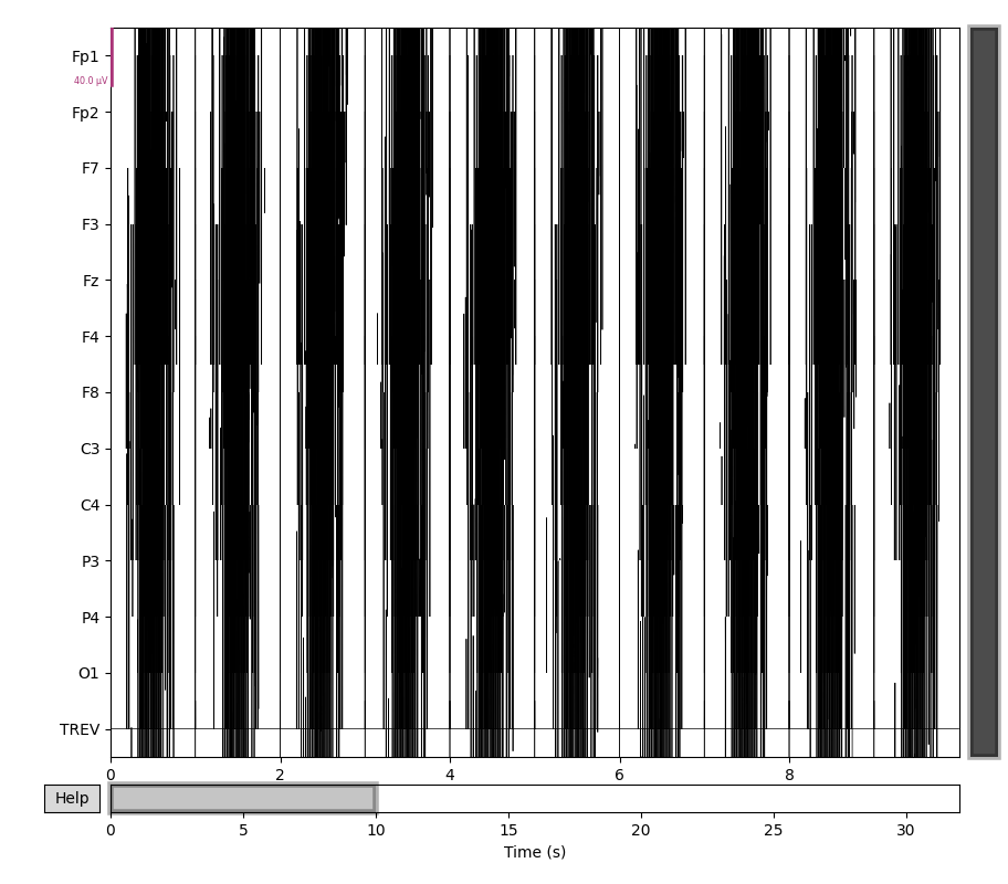
The gradient artifact dominates the recording – the underlying EEG signal is not visible at this scale.

raw.plot()

Remove the gradient artifact

remove_fmri_gradient_artifact() implements average artifact subtraction (AAS): for each TR, it builds a template by averaging neighboring TRs (window=(4, 4) here averages the 4 TRs before and the 4 TRs after) and subtracts it.

raw_clean = remove_fmri_gradient_artifact(raw, events, window=(4, 4))

Filter the cleaned data

With the (much larger) gradient artifact gone, a standard band-pass filter can be applied as usual.

filt = raw_clean.filter(l_freq=1.0, h_freq=30, n_jobs=2)

Filtering raw data in 1 contiguous segment
Setting up band-pass filter from 1 - 30 Hz

FIR filter parameters
---------------------
Designing a one-pass, zero-phase, non-causal bandpass filter:
- Windowed time-domain design (firwin) method
- Hamming window with 0.0194 passband ripple and 53 dB stopband attenuation
- Lower passband edge: 1.00
- Lower transition bandwidth: 1.00 Hz (-6 dB cutoff frequency: 0.50 Hz)
- Upper passband edge: 30.00 Hz
- Upper transition bandwidth: 7.50 Hz (-6 dB cutoff frequency: 33.75 Hz)
- Filter length: 3301 samples (3.301 s)

[Parallel(n_jobs=2)]: Using backend ThreadingBackend with 2 concurrent workers.
[Parallel(n_jobs=2)]: Done  12 out of  12 | elapsed:    0.0s finished

Visualize the result

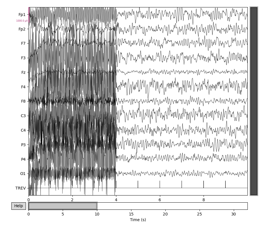
The recovered EEG signal is now visible at a realistic amplitude scale. The default per-channel scaling is tuned for real (much smaller) EEG artifacts, so we pass an explicit scalings value matched to our synthetic noise amplitude for a readable plot.

Note

The first 4 TRs are not cleaned, since they were needed to build the averaging template for artifact removal (window=(4, 4) looks 4 TRs ahead and behind). You can see the gradient artifact’s continued presence at the start of the plot below.

filt.plot(scalings=dict(eeg=500e-6))

See also

For simultaneous EEG-fMRI recordings, the gradient artifact is often removed first (as above), followed by removal of the cardiac (ballistocardiographic) artifact with mne.preprocessing.apply_pca_obs().

References

[1]

Philip J. Allen, Oliver Josephs, and Robert Turner. A method for removing imaging artifact from continuous EEG recorded during functional MRI. NeuroImage, 12(2):230–239, 2000. doi:10.1006/nimg.2000.0599.